CSC413 Neural Networks and Deep Learning

Lecture 2

Last Week

• Review of linear models
  • linear regression
  • linear classification (logistic regression)
• Gradient descent to train these models

This Week

• Biological and Artifical Neurons
• Limitations of Linear Models for Classification
• Multilayer Perceptrons
• Backpropagation

Biological and Artificial Neurons

Neuron

• A Neuron is a cell also known as nerve cell

Neuron Anatomy

• The dendrites, which are connected to other cells that provide information.
• The cell body, which consolidates information from the dendrites.
• The axon, which is an extension from the cell body that passes information to other cells.
• The synapse, which is the area where the axon of one neuron and the dendrite of another connect.

What does a neuron do?

• Consolidates “information” (voltage difference) from its dendrites
• If the total activity in a neuron’s dendrite lowers the voltage difference enough, the entire cell depolarizes and the neuron fires

What does a neuron do?

• The voltage signal spreads along the axon and to the synapse, then to the next neurons
• Neuron sends information to the next cell

What makes a neuron fire?

Neurons can fire in response to…

• retinal cells
• certain edges, lines, angles, movements
• hands and faces (in primates)
• specific people (in humans)
  • although the existence of these “grandmother cells” is contested

• Grandmother cells are also known as Jennifer Aniston neurons
• Observed single neuron firing when shown pictures of Jennifer Aniston by operating on patients with epileptic seizures.

Modeling Individual Neurons

• \(x_{i}\) are inputs to the neuron
• \(w_{i}\) are the neuron’s weights
• \(b\) is the neuron’s bias

• In Learning with Artifical Neural Networks, we want to create a simplified model of neurons in the brain.

Modeling Individual Neurons II

• \(f\) is an activation function
• \(f(\sum_i x_i w_i + b)\) is the neuron’s activation (output)

Linear Models as a Single Neuron

• \(x_{i}\) are the inputs
• \(w_{i}\) are components of the weight vector \({\bf w}\)
• \(b\) is the bias

• A (univariate) linear model can be interpreted as one single neuron.
• Univariate means that we model one single attribute.

Linear Models as a Single Neuron II

• \(f\) is the identity function
• \(y = \sum_i x_i w_i + b = {\bf w}^\top {\bf x} + b\) is the output

Logistic Regression Models (for Binary Classification) as a Single Neuron

• \(x_{i}\) are the inputs
• \(w_{i}\) are components of the weight vector \({\bf w}\)
• \(b\) is the bias

Logistic Regression Models (for Binary Classification) as a Single Neuron II

• \(f = \sigma\)
• \(y = \sigma(\sum_i x_i w_i + b) = \sigma({\bf w}^\top {\bf x} + b)\)

Logistic Regression Models (for Multi-Class Classification) as a Neural Network

We use \(K\) neurons (one for each class):

• \(x_{i}\) are the inputs
• \(w_{j,i}\) are components of the weight matrix \(W\in \mathbb{R}^{K\times N}\)
• \(b_i\) are components of the bias vector \({\bf b}\)
• \(f = \text{softmax}\) : applied to the entire vector of values
• \({\bf y} = \text{softmax}(W{\bf x} + {\bf b})\) : outputs of \(K\) neurons

• Now we have an entire weight matrix \(W\) with \(K\) rows and a \(K\)-dimensional bias vector. One for each class.

Limits of Linear Models for Binary Classification

XOR example

• Single neurons (linear classifiers) are very limited in expressive power
• XOR is a classic example of a function that’s not linearly separable, with an elegant proof using convexity

Convex Sets

A set \(S\subseteq\mathbb{R}^n\) is convex if any line segment connecting points in \(S\) lies in \(S\).

More formally, \(S\) is convex iff

\[{\bf x_1}, {\bf x_2} \in S \implies \forall \lambda \in [0,\, 1],\, \lambda {\bf x_1} + (1 - \lambda){\bf x_2} \in S.\]

A simple inductive argument shows that for \({\bf x_1}, \dots, {\bf x_N} \in S\), the weighted average or convex combination lies in the set:

\[\lambda_1 {\bf x_1} + \dots + \lambda_N {\bf x_N} \in S \text{ for }\lambda_1 + \dots + \lambda_N = 1\ .\]

• iff stands for “if and only if”

XOR not linearly separable

Initial Observations

• A binary linear classifier divides the euclidean space into two half-spaces
• Half-spaces are convex

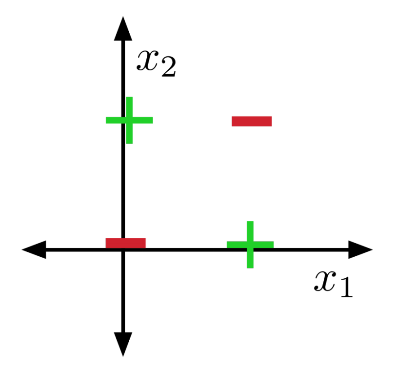
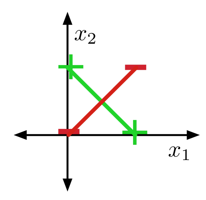
XOR not linearly separable II

• Suppose there were some feasible hypothesis. If the positive examples are in the positive half-space, then the green line segment must be as well.
• Similarly, red line segment must lie within the negative half-space.
• But the intersection can’t lie in both half-spaces. Contradiction!

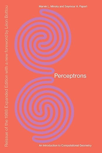
History of the XOR Example

• Minsky and Papert shown in their work Perceptrons that XOR cannot be learned by a Neuron.
• Its pessimistic outlook on perceptrons is assumed as one of the causes for the AI winter of the 70s / early 80s.

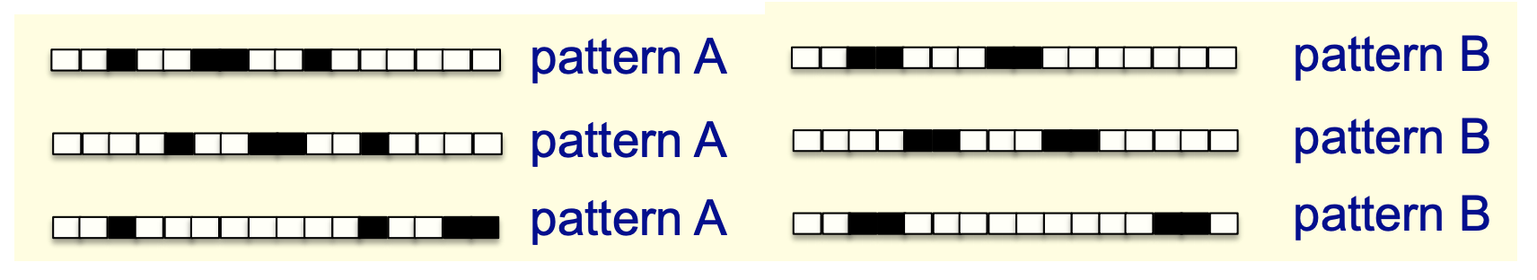
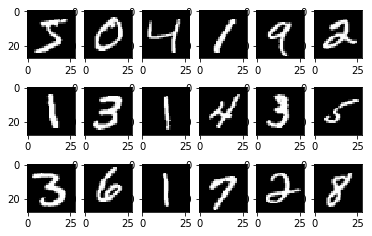
A more troubling example

These images represent 16-dimensional vectors. Want to distinguish patterns A and B in all possible translations (with wrap-around).

Suppose there’s a feasible solution. The average of all translations of A is the vector (0.25, 0.25, . . . , 0.25). Therefore, this point must be classified as A. All translations of B have the same average. Contradiction!

• The argument here is basically a convexity argument again
• The average of all possible patterns A must be classified as A because of convexity. Same for B
• However, both patterns have the same average leading to a contradiction

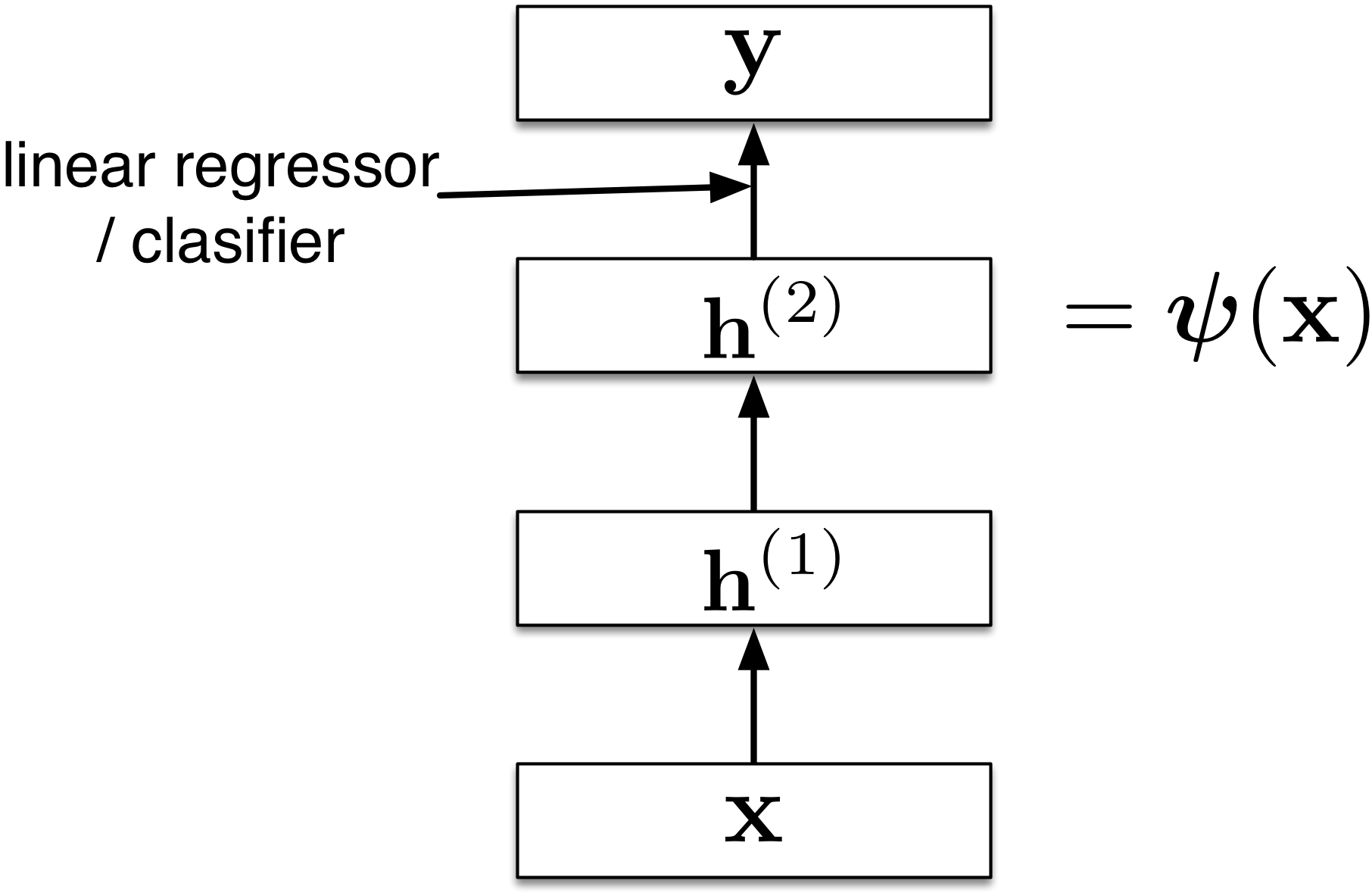
(Nonlinear) Feature Maps

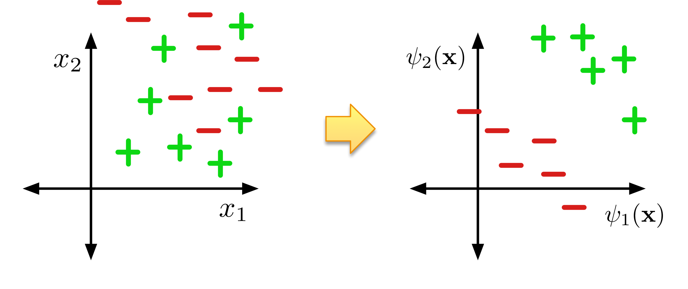
Sometimes, we can overcome this limitation with nonlinear feature maps.

Nonlinear feature maps transform the original input features into a different (often higher dimensional) representation.

Consider the XOR problem again and use the following feature map: \[\Psi({\bf x}) = \begin{pmatrix}x_1 \\ x_2 \\ x_1x_2 \end{pmatrix}\]

(Nonlinear) Feature Maps II

\(x_1\)	\(x_2\)	\(\phi_1({\bf x})\)	\(\phi_2({\bf x})\)	\(\phi_3({\bf x})\)	t
0	0	0	0	0	0
0	1	0	1	0	1
1	0	1	0	0	1
1	1	1	1	1	0

This is linearly separable (Try it!)

… but generally, it can be hard to pick good basis functions.

We’ll use neural nets to learn nonlinear hypotheses directly

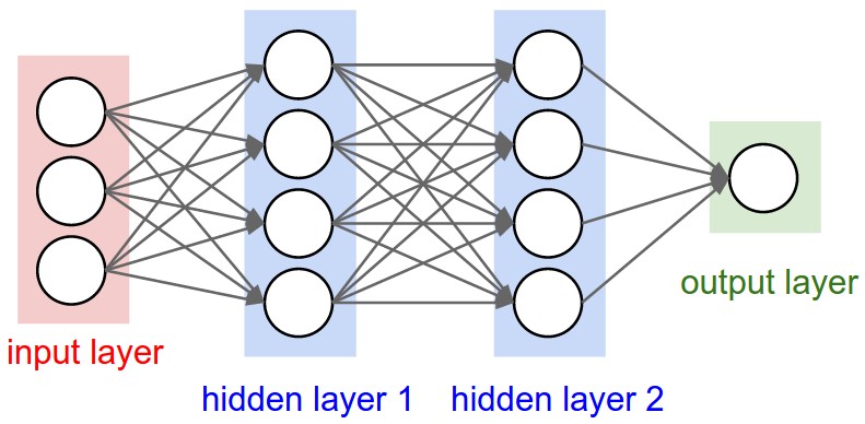
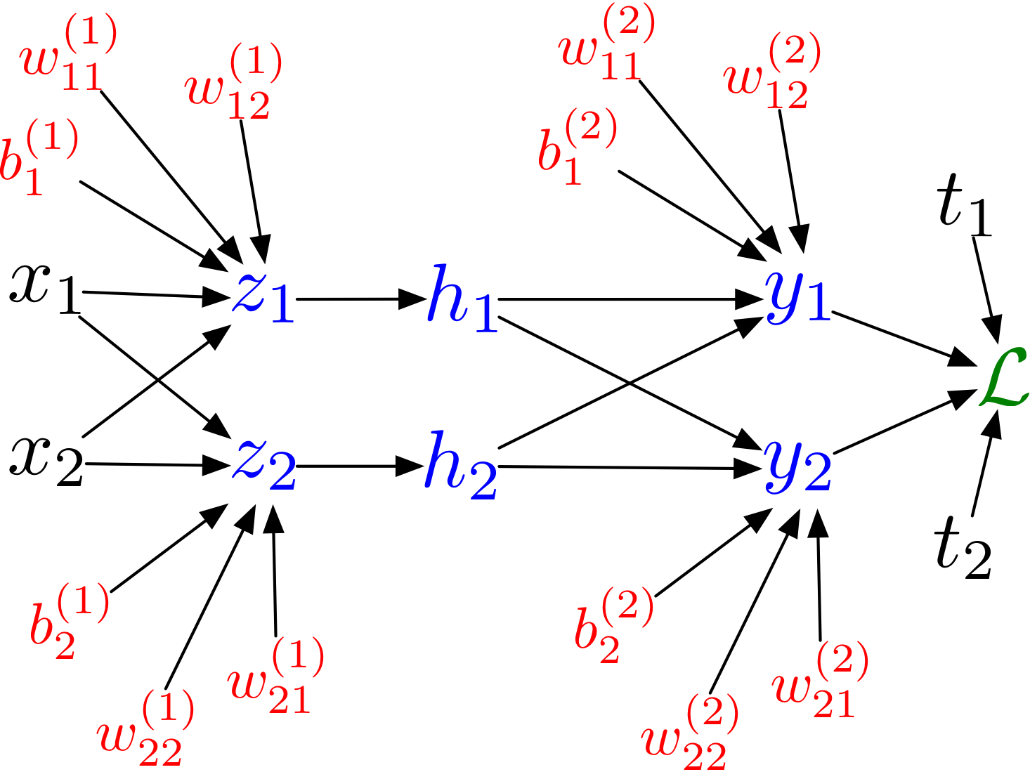
Multilayer Perceptrons

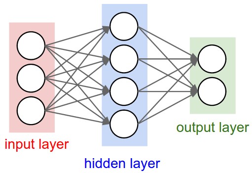
An Artificial Neural Network (Multilayer Perceptron)

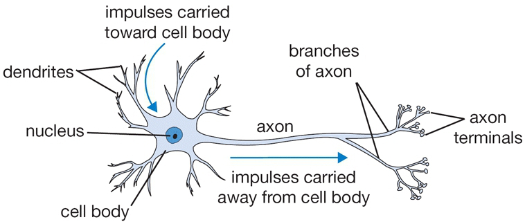
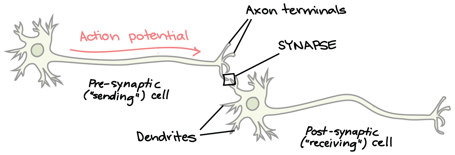
Idea

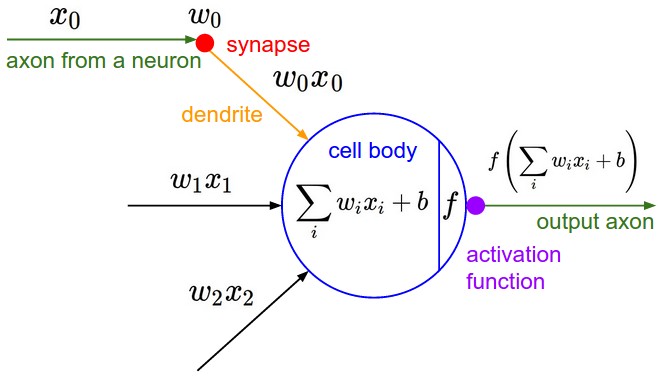
• Use a simplified (mathematical) model of a neuron as building blocks
• Connect the neurons together accross multiple layers.

An Artificial Neural Network (Multilayer Perceptron) II

• An input layer: feed in input features (e.g. like retinal cells in your eyes)
• A number of hidden layers: don’t have specific meaning
• An output layer: interpret output like a “grandmother cell”

But what do these neurons mean?

• Use \(x_i\) to encode the input
  • e.g. pixels in an image

• Use \(y\) to encode the output (of a binary classification problem)
  • e.g. cancer vs. not cancer

• Use \(h_i^{(k)}\) to denote a unit in the hidden layer
  • difficult to interpret

• \(x_i\) can be thought of as the neurons that are connected to the receptors in the eye
• \(y\) can be thought of as a grandmother cell.

Example: MNIST Digit Recognition

MNIST Digit Recognition II

With a logistic regression model, we would have:

• Input: An 28x28 pixel grayscale image
  • \({\bf x}\) is a vector of length 784

• Target: The digit represented in the image
  • \({\bf t}\) is a one-hot vector of length 10

• Model: \({\bf y} = \text{softmax}(W{\bf x} + {\bf b})\)

• Each \(x_i\) is a intensity value of the corresponding pixel, i.e. a value between 0 and 255.
• As a reminder: the one-hot vector has 1 at the entry corresponding to the classified number and 0 everywhere elese.

Adding a Hidden Layer

Two layer neural network

• Input size: 784 (number of features)
• Hidden size: 50 (we choose this number)
• Output size: 10 (number of classes)

• All the numbers that we can choose such as the number of hidden units are known as Hyperparameters.

Side note about machine learning models

When discussing machine learning and deep learning models, we usually

• first talk about how to make predictions assume the weights are trained
• then talk about how to train the weights

Often the second step requires gradient descent or some other optimization method

Making Predictions: computing the hidden layer

\[\begin{align*} h_1 &= f\left(\sum_{i=1}^{784} w^{(1)}_{1,i} x_i + b^{(1)}_1\right) \\ h_2 &= f\left(\sum_{i=1}^{784} w^{(1)}_{2,i} x_i + b^{(1)}_2\right) \\ ... \end{align*}\]

Making Predictions: computing the output (pre-activation)

\[\begin{align*} z_1 &= \sum_{j=1}^{50} w^{(2)}_{1,j} h_j + b^{(2)}_1 \\ z_2 &= \sum_{j=1}^{50} w^{(2)}_{2,j} h_j + b^{(2)}_2 \\ ... \end{align*}\]

Making Predictions: applying the output activation

\[\begin{align*} {\bf z} &= \begin{bmatrix}z_1 \\ z_2 \\ \vdots \\ z_{10}\end{bmatrix},\quad {\bf y} = \text{softmax}({\bf z}) \end{align*}\]

Making Predictions: Vectorized

\[\begin{align*} {\bf h} &= f(W^{(1)}{\bf x} + {\bf b}^{(1)}) \\ {\bf z} &= W^{(2)}{\bf h} + {\bf b}^{(2)} \\ {\bf y} &= \text{softmax}({\bf z}) \end{align*}\]

Activation Functions: common choices

Common Choices:

• Sigmoid activation
• Tanh activation
• ReLU activation

Rule of thumb: Start with ReLU activation. If necessary, try tanh.

Activation Function: Sigmoid

• Gradient vanishes at the extremes as the function converges to \(0\) and \(1\) respectively.
• All activations are positive (see this blog post to learn why we don’t want this)

• Having only positive activations can lead to undesired behavior during training because all weights entering a neuron can either be only increased or only decreased.

Activation Function: Tanh

• scaled version of the sigmoid activation
• also somewhat problematic due to gradient signal
• activations can be positive or negative

Activation Function: ReLU

• most often used nowadays
• all activations are positive
• easy to compute gradients
• can be problematic if the bias is too large and negative, so the activations are always 0

• The last point is known as the dying ReLU phenomenon if a neuron becomes inactive and never recovers.

Feature Learning

Neural nets can be viewed as a way of learning features:

Feature Learning (cont’d)

The goal is for these features to become linearly separable:

Computing XOR

Exercise: design a network to compute XOR

Use a hard threshold activation function:

\[\begin{align*} f(x) = \begin{cases} 1, & x \geq 0 \\ 0, & x < 0 \end{cases} \end{align*}\]

Computing XOR Demo

Demo: https://playground.tensorflow.org/

Expressive Power: Linear Layers (No Activation Function)

• We’ve seen that there are some functions that linear classifiers can’t represent. Are deep networks any better?
• Any sequence of layers (with no activation function) can be equivalently represented with a single linear layer.

\[\begin{align*} {\bf y} &= \left(W^{(3)} W^{(2)} W^{(1)}\right) {\bf x} \\ &= W^\prime {\bf x} \end{align*}\]

Deep linear networks are no more expressive than linear regression!

Expressive Power: MLP (nonlinear activation)

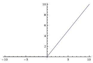
• Multilayer feed-forward neural nets with nonlinear activation functions are universal approximators: they can approximate any function arbitrarily well.
• This has been shown for various activation functions (thresholds, logistic, ReLU, etc.)
  • Even though ReLU is “almost” linear, it’s nonlinear enough!

Universality for binary inputs and targets

• Hard threshold hidden units, linear output
• Strategy: \(2^D\) hidden units, each of which responds to one particular input configuration
  • Only requires one hidden layer, though it needs to be extremely wide!

Limits of universality

• You may need to represent an exponentially large network.
• If you can learn any function, you might just overfit.

• As an exercise: try to think how such units would look like.

Backpropagation

Training Neural Networks

• How do we find good weights for the neural network?
• We can continue to use the loss functions:
  • cross-entropy loss for classification
  • square loss for regression
• The neural network operations we used (weights, etc) are (almost everywhere) differentiable

We can use gradient descent!

Gradient Descent Recap

Goal: Compute the minimum of a function \(\mathcal{E}({\bf a})\)

• Start with a set of parameters \(\mathbf{a}_0\) (initialize to some value)
• Compute the gradient \(\frac{\partial \mathcal{E}}{\partial \mathbf{a}}\).
• Update the parameters towards the negative direction of the gradient

Gradient Descent for Neural Networks

Idea: Use gradient descent for “learning” neural networks.

• We have a lot of parameters
  • High dimensional (all weights and biases are parameters)
  • Hard to visualize
  • Many iterations (“steps”) needed
• In Deep Learning \(\frac{\partial \mathcal{E}}{\partial w}\) is the average of \(\frac{\partial \mathcal{L}}{\partial w}\) over multiple training examples

Challenge: How to compute \(\frac{\partial \mathcal{L}}{\partial w}\) effectively.

Solution: Backpropagation!

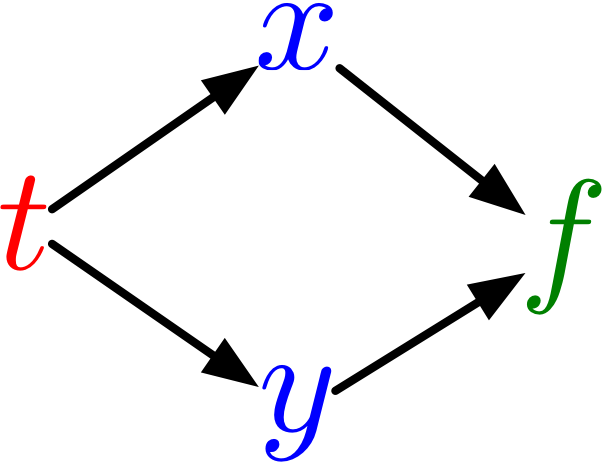
Univariate Chain Rule

Recall: if \(f(x)\) and \(x(t)\) are univariate functions, then

\[\frac{d}{dt}f(x(t)) = \frac{df}{dx}\frac{dx}{dt}\]

Univariate Chain Rule for Least Squares with a Logistic Model

Recall: Univariate logistic least squares model

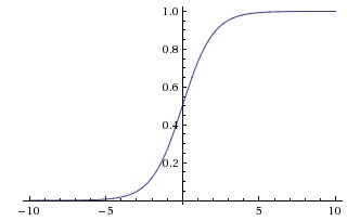
\[\begin{align*} z &= wx + b \\ y &= \sigma(z) \\ \mathcal{L} &= \frac{1}{2}(y - t)^2 \end{align*}\]

Let’s compute the loss derivative

Univariate Chain Rule Computation I

How you would have done it in calculus class

\[\begin{align*} \mathcal{L} &= \frac{1}{2} ( \sigma(w x + b) - t)^2 \\ \frac{\partial \mathcal{L}}{\partial w} &= \frac{\partial}{\partial w} \left[ \frac{1}{2} ( \sigma(w x + b) - t)^2 \right] \\ &= \frac{1}{2} \frac{\partial}{\partial w} ( \sigma(w x + b) - t)^2 \\ &= (\sigma(w x + b) - t) \frac{\partial}{\partial w} (\sigma(w x + b) - t) \\ &\ldots \end{align*}\]

Univariate Chain Rule Computation II

How you would have done it in calculus class

\[\begin{align*} \ldots &= (\sigma(w x + b) - t) \frac{\partial}{\partial w} (\sigma(w x + b) - t) \\ &= (\sigma(w x + b) - t) \sigma^\prime (w x + b) \frac{\partial}{\partial w} (w x + b) \\ &= (\sigma(w x + b) - t) \sigma^\prime (w x + b) x \end{align*}\]

Univariate Chain Rule Computation III

Similarly for \(\frac{\partial \mathcal{L}}{\partial b}\)

\[\begin{align*} \mathcal{L} &= \frac{1}{2} ( \sigma(w x + b) - t)^2 \\ \frac{\partial \mathcal{L}}{\partial b} &= \frac{\partial}{\partial b} \left[ \frac{1}{2} ( \sigma(w x + b) - t)^2 \right] \\ &= \frac{1}{2} \frac{\partial}{\partial b} ( \sigma(w x + b) - t)^2 \\ &= (\sigma(w x + b) - t) \frac{\partial}{\partial b} (\sigma(w x + b) - t) \\ &\ldots \end{align*}\]

Univariate Chain Rule Computation IV

Similarly for \(\frac{\partial \mathcal{L}}{\partial b}\)

\[\begin{align*} \ldots &= (\sigma(w x + b) - t) \frac{\partial}{\partial b} (\sigma(w x + b) - t) \\ &= (\sigma(w x + b) - t) \sigma^\prime (w x + b) \frac{\partial}{\partial b} (w x + b) \\ &= (\sigma(w x + b) - t) \sigma^\prime (w x + b) \end{align*}\]

Q: What are the disadvantages of this approach?

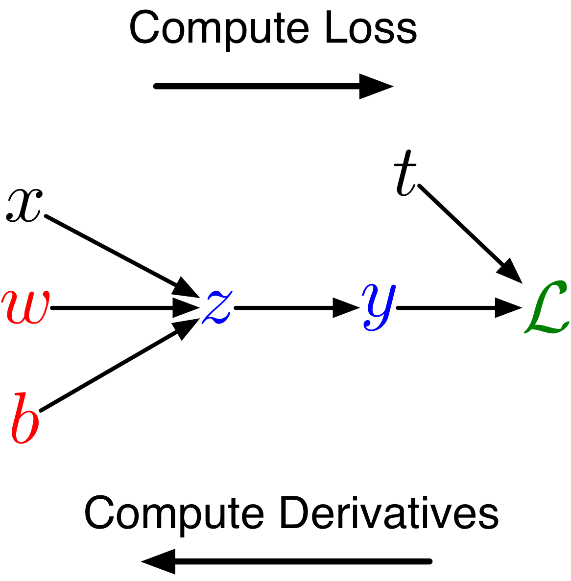
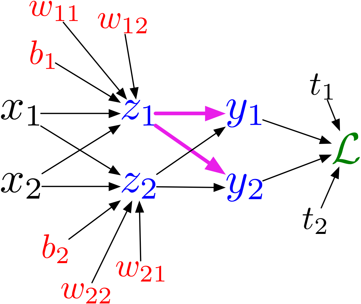
A More Structured Way to Compute the Derivatives

\[\begin{align*} z &= wx + b \\ y &= \sigma(z) \\ \mathcal{L} &= \frac{1}{2}(y - t)^2 \end{align*}\]

Less repeated work; easier to write a program to efficiently compute derivatives

A More Structured Way to Compute the Derivatives II

\[\begin{align*} \frac{d \mathcal{L}}{d y} &= y - t \\ \frac{d \mathcal{L}}{d z} &= \frac{d \mathcal{L}}{d y}\sigma'(z) \\ \frac{\partial \mathcal{L}}{\partial w} &= \frac{d \mathcal{L}}{d z} \, x \\ \frac{\partial \mathcal{L}}{\partial b} &= \frac{d \mathcal{L}}{d z} \end{align*}\]

Less repeated work; easier to write a program to efficiently compute derivatives

Computation Graph

We can diagram out the computations using a computation graph.

• The nodes represent all the inputs and computed quantities.
• The edges represent which nodes are computed directly as a function of which other nodes.

Chain Rule (Error Signal) Notation

• Use \(\overline{y}\) to denote the derivative \(\frac{d \mathcal{L}}{d y}\)
  • sometimes called the error signal
• This notation emphasizes that the error signals are just values our program is computing (rather than a mathematical operation).
• This is notation introduced by Prof. Roger Grosse, and not standard notation

Chain Rule (Error Signal) Notation II

Computing the loss:

\[\begin{align*} z &= wx + b \\ y &= \sigma(z) \\ \mathcal{L} &= \frac{1}{2}(y - t)^2 \end{align*}\]

Computing the derivatives:

\[\begin{align*} \overline{y} &= y - t \\ \overline{z} &= \overline{y} \sigma'(z) \\ \overline{w} &= \overline{z} \, x \\ \overline{b} &= \overline{z} \end{align*}\]

Multiclass Logistic Regression Computation Graph

In general, the computation graph fans out:

Multiclass Logistic Regression Computation Graph II

\[\begin{align*} z_l &= \sum_j w_{lj} x_j + b_l \\ y_k &= \frac{e^{z_k}}{\sum_l e^{z_l}} \\ \mathcal{L} &= -\sum_k t_k \log{y_k} \end{align*}\]

There are multiple paths for which a weight like \(w_{11}\) affects the loss \(\mathcal{L}\).

Multivariate Chain Rule

Suppose we have a function \(f(x, y)\) and functions \(x(t)\) and \(y(t)\) (all the variables here are scalar-valued). Then

\[\frac{d}{dt}f(x(t), y(t)) = \frac{\partial f}{\partial x}\frac{dx}{dt} + \frac{\partial f}{\partial y}\frac{dy}{dt}\]

Multivariate Chain Rule Example

If \(f(x, y) = y + e^{xy}\), \(x(t) = \cos t\) and \(y(t) = t^2\)…

\[\begin{align*} \frac{d}{dt}f(x(t), y(t)) &= \frac{\partial f}{\partial x}\frac{dx}{dt} + \frac{\partial f}{\partial y}\frac{dy}{dt} \\ &= \left( y e^{xy} \right) \cdot \left( -\sin (t) \right) + \left( 1 + xe^{xy} \right) \cdot 2t \end{align*}\]

Multivariate Chain Rule Notation

In our notation

\[\overline{t} = \overline{x} \frac{dx}{dt} + \overline{y} \frac{dy}{dt}\]

The Backpropagation Algorithm

• Backpropagation is an algorithm to compute gradients efficiency
  • Forward Pass: Compute predictions (and save intermediate values)
  • Backwards Pass: Compute gradients
• The idea behind backpropagation is very similar to dynamic programming
  • Use chain rule, and be careful about the order in which we compute the derivatives

Backpropagation Example

Backpropagation for a MLP

Forward pass: \[\begin{align*} z_i &= \sum_j w_{ij}^{(1)} x_j + b_i^{(1)} \\ h_i &= \sigma(z_i) \\ y_k &= \sum_i w_{ki}^{(2)} h_i + b_k^{(2)} \\ \mathcal{L} &= \frac{1}{2}\sum_k (y_k - t_k)^2 \end{align*}\]

Backpropagation for a MLP II

Backward pass:

\[\begin{align*} \overline{\mathcal{L}} &= 1 \\ \overline{y_k} &= \overline{\mathcal{L}}(y_k - t_k) \\ \overline{w_{ki}^{(2)}} &= \overline{y_k}h_i \\ \overline{b_{k}^{(2)}} &= \overline{y_k} \end{align*}\]

\[\begin{align*} \overline{h_i} &= \sum_k \overline{y_k} w_{ki}^{(2)} \\ \overline{z_i} &= \overline{h_i} \sigma'(z_i) \\ \overline{w_{ij}^{(1)}} &= \overline{z_i} x_j \\ \overline{b_{i}^{(1)}} &= \overline{z_i} \end{align*}\]

Backpropagation for a MLP

Forward pass: \[\begin{align*} {\bf z} &= W^{(1)}{\bf x} + {\bf b}^{(1)} \\ {\bf h} &= \sigma({\bf z}) \\ {\bf y} &= W^{(2)}{\bf h} + {\bf b}^{(2)} \\ \mathcal{L} &= \frac{1}{2} || {\bf y} - {\bf t}||^2 \end{align*}\]

Backpropagation for a MLP

Backward pass: \[\begin{align*} \overline{\mathcal{L}} &= 1 \\ \overline{{\bf y}} &= \overline{\mathcal{L}}({\bf y} - {\bf t}) \\ \overline{W^{(2)}} &= \overline{{\bf y}}{\bf h}^\top \\ \overline{{\bf b^{(2)}}} &= \overline{{\bf y}} \\ & \ldots \end{align*}\]

Backpropagation for a MLP

Backward pass: \[\begin{align*} & \ldots \\ \overline{{\bf h}} &= {W^{(2)}}^\top\overline{y} \\ \overline{{\bf z}} &= \overline{{\bf h}} \circ \sigma'({\bf z}) \\ \overline{W^{(1)}} &= \overline{{\bf z}} {\bf x}^\top \\ \overline{{\bf b}^{(1)}} &= \overline{{\bf z}} \end{align*}\]

Implementing Backpropagation I

Implementing Backpropagation II

Forward pass: Each node…

• receives messages (inputs) from its parents
• uses these messages to compute its own values

Backward pass: Each node…

• receives messages (error signals) from its children
• uses these messages to compute its own error signal
• passes message to its parents

This algorithm provides modularity!

Backpropagation in Vectorized Form

Backpropagation in practice

• Backprop is used to train the overwhelming majority of neural nets today.
  • Even optimization algorithms much fancier than gradient descent (e.g.~second-order methods) use backprop to compute the gradients.

Backpropagation in practice II

• Despite its practical success, backprop is believed to be neurally (biologically) implausible.
  • No evidence for biological signals analogous to error derivatives.
  • All the biologically plausible alternatives we know about learn much more slowly (on computers).

Wrap Up

Summary

• Artificial neurons draw inspiration from nerve cells / neurons in the brain
• On its own, the expresiveness of a single neuron is limited
• Stacking neurons and nonlinear activation functions allows for learning more complex functions
• Backpropagation can be used for this learning task

What to do this week?

• You can already complete Assignment 1
  • Start early so you can get help early!
• Attend tutorials this week!
• Complete the readings for this week.
• Preview next week’s materials