CSC413 Neural Networks and Deep Learning

Lecture 4

Lecture Overview

Last Week

• Automatic differentiation
• Distributed representations
• GloVe embeddings

This week

• Computer Vision
• Convolutional Layers
• Downsampling
• Training a ConvNet
• Examples and Applications

Computer Vision

Computer vision is hard

• In 2012, when Deep Learning had its most recent comeback it was because of computer vision.
• Object change in pose, size, viewpoint, background, illumination
• Some objects are hidden behind others: occlusion

Computer vision is really hard

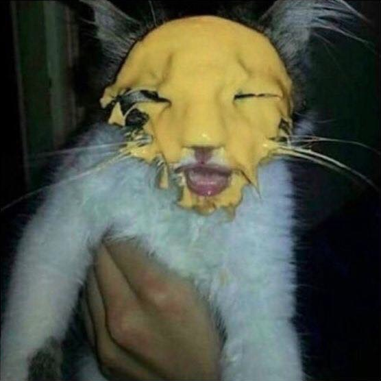
How can you “hard code” an algorithm that still recognizes that this is a cat?

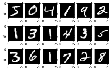
Working with Small Images

In the week 3 tutorial, we worked with small, MNIST images, which are \(28 \times 28\) pixels, black and white.

How do our models work?

Notebook Demo - Logistic Regression Weights

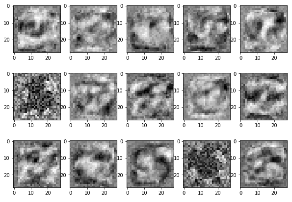
Notebook Demo - MLP Weights (first layer)

Working with Large Images

• Suppose you have an image that is 200 pixels x 200 pixels
• There are 500 units in the first hidden layer

Q: How many parameters will there be in the first layer?

A: \(200 \times 200 \times 500 + 500 =\) over 20 million!

Working with Large Images II

Q: Why might using a fully connected layer be problematic?

• computing predictions (forward pass) will take a long time
• large number of weights requires a lot of training data to avoid overfitting
• small shift in image can result in large change in prediction

Convolutional Layers

Biological Influence

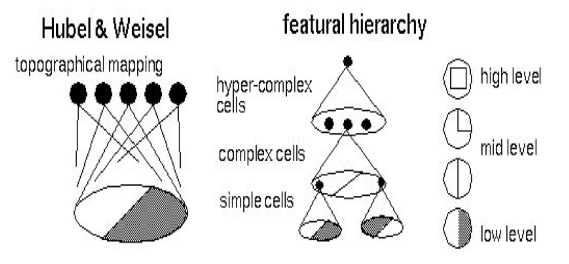
There is evidence that biological neurons in the visual cortex have locally-connected connections

See Hubel and Wiesel Cat Experiment (Note: there is an anesthetised cat in the video that some may find disturbing).

• Harvard neurophysiologists David H. Hubel / Torsten Wiesel
• Inserted a microelectrode into primary visual cortex of a cat.
• Projected patterns of light and dark on a screen in front of the cat
• Found that some neurons fired rapidly when presented with lines at one angle, while others responded best to another angle.
• More on this here

Convolutional Neural Network

• Locally-connected layers: compute local features based on small regions of the image
  • Examples of features:
    • a horizontal edge in an area
    • a vertical edge in an area
    • a blob (no edges) in the area
    • a circular shape in the area
• Weight-sharing: detect the same local features across the entire image

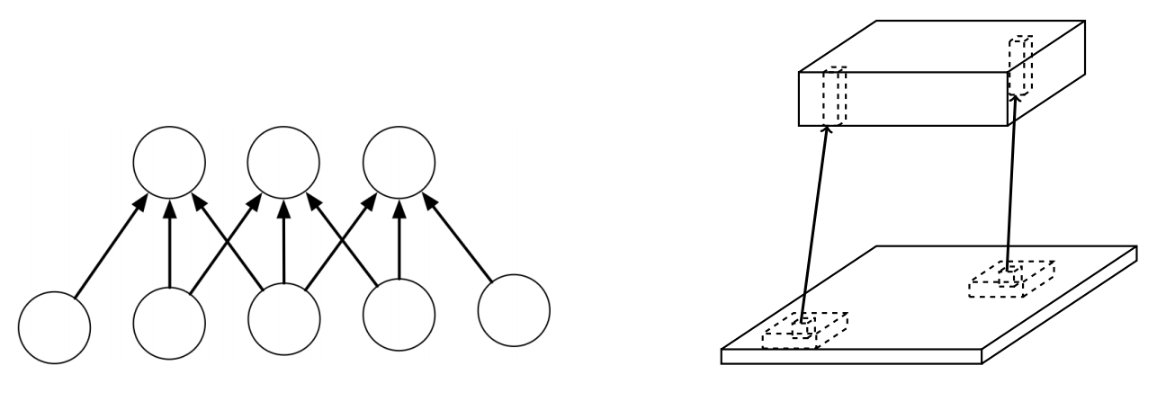
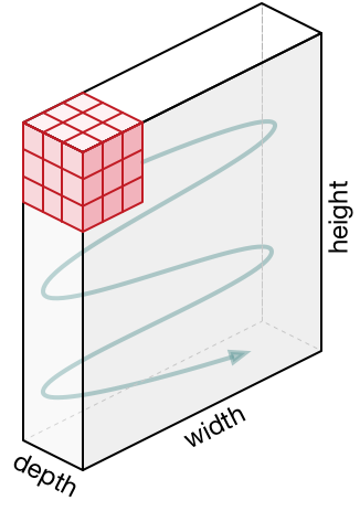
Locally Connected Layers

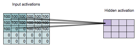
Each hidden unit connects to a small region of the input (in this case a \(3 \times 3\) region)

Locally Connected Layers

(Remove lines for readability)

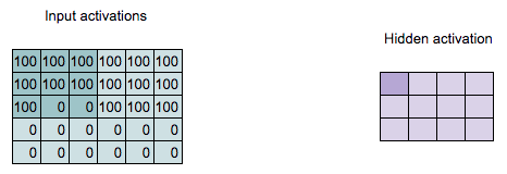
Locally Connected Layers

Hidden unit geometry has a 2D geometry consistent with the input.

Locally Connected Layers

Locally Connected Layers

Locally Connected Layers

Locally Connected Layers

Locally Connected Layers

Q: Which region of the input is this hidden unit connected to?

Locally Connected Layers

Summary

Fully-connected layers:

Locally connected layers:

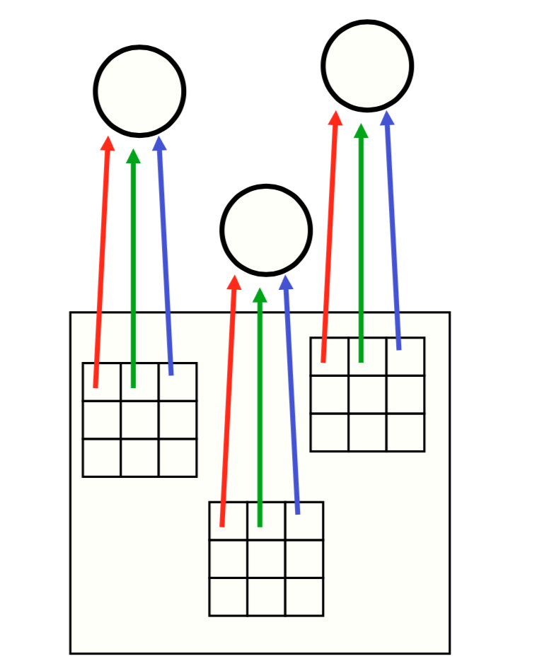
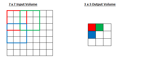
Weight Sharing

Locally connected layers

Convolutional layers

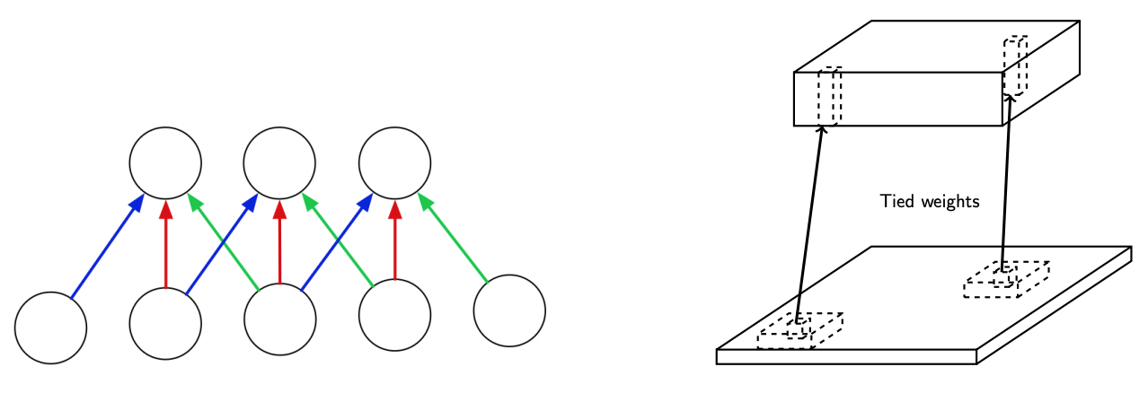
Use the same weights across each region (each colour represents the same weight)

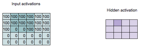
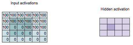
Convolution Computation

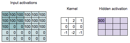
\[\begin{align*} 300 = & 100 \times 1 + 100 \times 2 + 100 \times 1 + \\ & 100 \times 0 + 100 \times 0 + 100 \times 0 + \\ & 100 \times (-1) + 0 \times (-2) + 0 \times (-1) \end{align*}\]

Convolution Computation II

\[\begin{align*} 300 = & 100 \times 1 + 100 \times 2 + 100 \times 1 + \\ & 100 \times 0 + 100 \times 0 + 100 \times 0 + \\ & 100 \times (-1) + 0 \times (-2) + 0 \times (-1) \end{align*}\]

• The kernel or filter (middle) contains the trainable weights
• In our example, the kernel size is \(3\times3\)
• The “convolved features” is another term for the output hidden activation

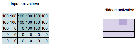
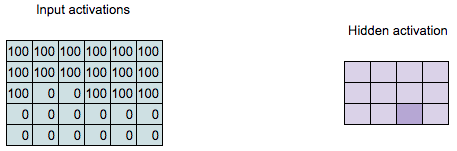
Convolution Computation

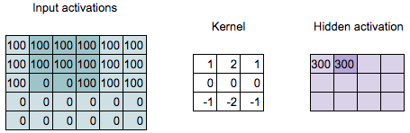
\[\begin{align*} 300 = &100 \times 1 + 100 \times 2 + 100 \times 1 + \\ &100 \times 0 + 100 \times 0 + 100 \times 0 + \\ &0 \times (-1) + 0 \times (-2) + 100 \times (-1) \end{align*}\]

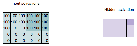
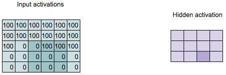
Convolution Computation

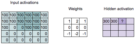
Q: What is the value of the highlighted hidden activation?

• Pause here and try to solve this for yourself.

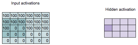
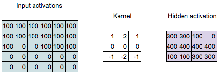
Convolution Computation

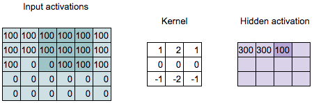
\[\begin{align*} 100 = &100 \times 1 + 100 \times 2 + 100 \times 1 + \\ &100 \times 0 + 100 \times 0 + 100 \times 0 + \\ &0 \times (-1) + 100 \times (-2) + 100 \times (-1) \end{align*}\]

Convolution Computation

Weight Sharing

Each neuron on the higher layer is detecting the same feature, but in different locations on the lower layer

“Detecting” = output (activation) is high if feature is present “Feature” = something in a part of the image, like an edge or shape

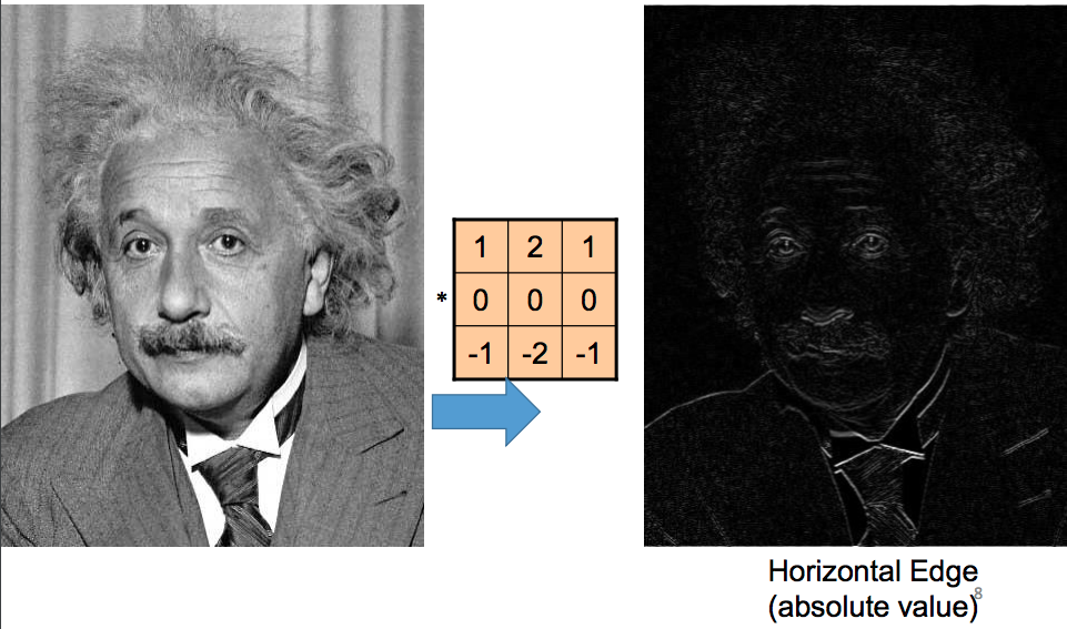
Sobel Filter - Weights to Detect Horizontal Edges

• The kernel we have seen in the previous example is commonly used to detect horizontal edges.
• It is known as the Sobel Filter or Sobel Operator

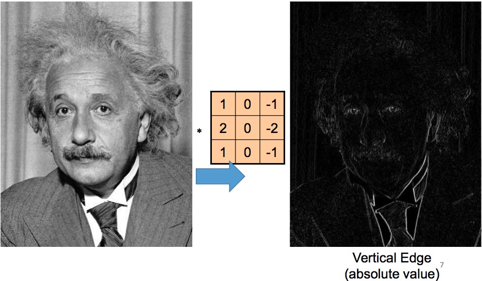
Sobel Filter - Weights to Detect Vertical Edges

• There is another kernel for vertical edges.

Weights to Detect Blobs

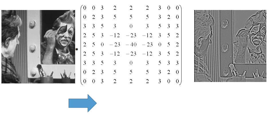
Q: What is the kernel size of this convolution?

• Blob detection is the task that aims at detecting regions of an image that differ from its surroundings.
• This can involve e.g. brightness or color.
• Here, the kernel is of size \(9\times 9\)

Example:

Greyscale input image: \(7\times 7\)

Convolution kernel: \(3 \times 3\)

Q: How many hidden units are in the output of this convolution?

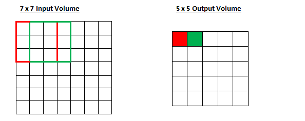
Q: How many trainable weights are there?

There are \(3 \times 3 + 1\) trainable weights (\(+ 1\) for the bias)

Convolutions in Practice

What if we have a coloured image?

What if we want to compute multiple features?

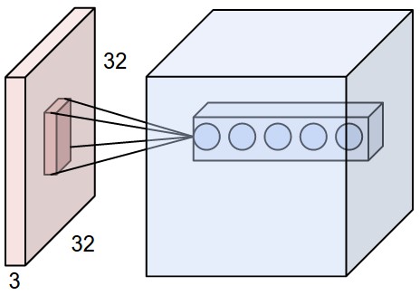
Convolution in RGB

The kernel becomes a 3-dimensional tensor!

In this example, the kernel has size 3 \(\times 3 \times 3\)

Convolutions: RGB Input

Colour input image: 3 \(\times 7 \times 7\)

Convolution kernel: 3 \(\times 3 \times 3\)

Questions:

• How many units are in the output of this convolution?
• How many trainable weights are there?

Terminology

Input image: \(3 \times 32 \times 32\)

Convolution kernel: 3 \(\times 3 \times 3\)

• The number 3 is the number of input channels or input feature maps

Detecting Multiple Features

Q: What if we want to detect many features of the input? (i.e. both horizontal edges and vertical edges, and maybe even other features?)

A: Have many convolutional filters!

Many Convolutional Filters

Input image: \(3 \times 7\times 7\)

Convolution kernel: \(3 \times 3 \times 3 \times\) 5

Q:

• How many units are in the output of this convolution?
• How many trainable weights are there?

More Terminology

Input image of size \(3 \times 32 \times 32\)

Convolution kernel of 3 \(\times 3 \times 3 \times\) 5

• The number 3 is the number of input channels or input feature maps
• The number 5 is the number of output channels or output feature maps

Example

Input features: \(5 \times 32 \times 32\)

Convolution kernel: \(5 \times 3 \times 3 \times 10\)

Questions:

• How many input channels are there?
• How many output channels are there?
• How many units are in the higher layer?
• How many trainable weights are there?

• Modern deep learning frameworks have all of this implemented.
• Still important to know as you design your network.

Downsampling

Consolidating Information

In a neural network with fully-connected layers, we reduced the number of units in each hidden layer

Q: Why?

• To be able to consolidate information, and remove out information not useful for the current task

Q: How can we consolidate information in a neural network with convolutional layers?

• max pooling, average pooling, strided convolutions

Max-Pooling

Idea: take the maximum value in each \(2 \times 2\) grid.

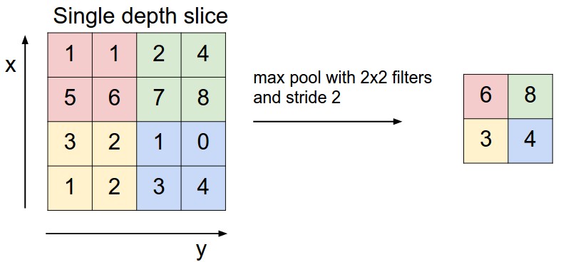
Max-Pooling Example

We can add a max-pooling layer after each convolutional layer

Average Pooling

• Average pooling (compute the average activation of a region)
• Max pooling generally works better

Strided Convolution

More recently people are doing away with pooling operations, using strided convolutions instead:

Shift the kernel by 2 (stride=2) when computing the next output feature.

Visualization examples

• https://arxiv.org/pdf/1603.07285.pdf
• https://github.com/vdumoulin/conv_arithmetic

Training a Conv Net

How do we train a conv net?

With backprop, of course!

Recall what we need to do. Backprop is a message passing procedure, where each layer knows how to pass messages backwards through the computation graph. Let’s determine the updates for convolution layers.

How do we train a conv net? II

• We assume we are given the loss derivatives \(\overline{y_{i,t}}\) with respect to the output units.
• We need to compute the cost derivatives with respect to the input units and with respect to the weights.

The only new feature is: how do we do backprop with tied weights?

• The derivatives with respect of the input units are not needed for the first layer
• But they are needed for all subsequent layers as the inputs to these subsequent layers are a function of previous layers’ weights.

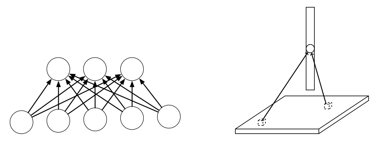
Multivariate Chain Rule (inputs)

Consider the computation graph for the inputs:

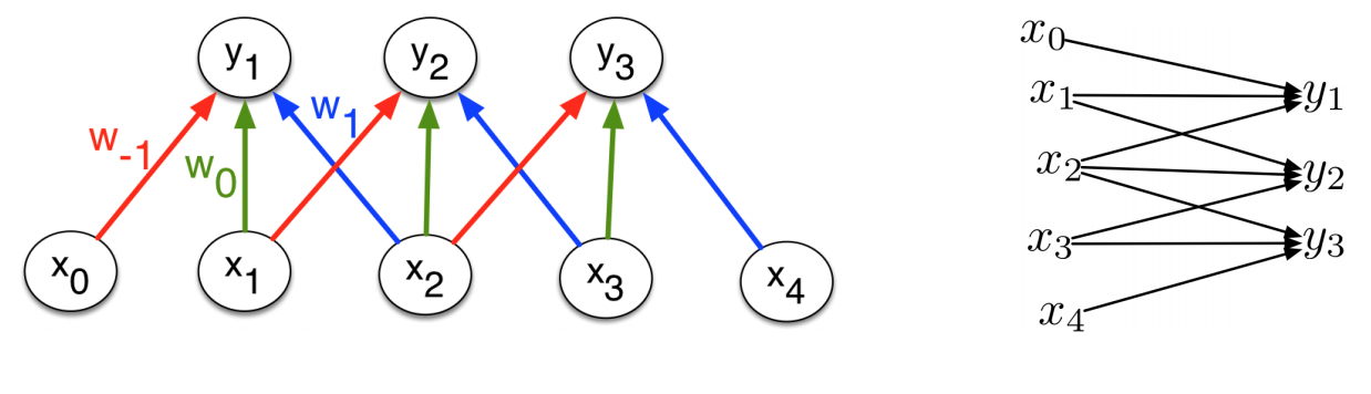
Each input unit influences all the output units that have it within their receptive fields. Using the multivariate Chain Rule, we need to sum together the derivative terms for all these edges

• This is a 1d signal, e.g. think of a 1d image with a line camera
• Here we have “kernels” of size 3
• We already applied multivariate chain rule for “tied inputs” in the past

Multivariate Chain Rule (weights)

Consider the computation graph for the weights:

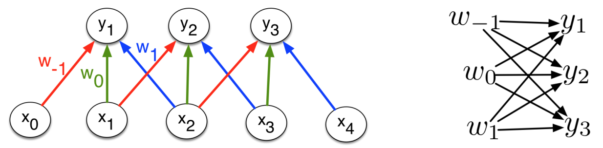
Each of the weights affects all the output units for the corresponding input and output feature maps.

Backpropagation on conv layers

The formula for the convolution layer for 1-D signals:

\[ y_{i,t} = \sum_{j=1}^{J} \sum_{\tau = -R}^{R} w_{i,j,\tau} \, x_{j, t + \tau}. \]

We compute the derivatives, which requires summing over all spatial locations:

\[\begin{align*} \overline{w_{i,j,\tau}} &= \sum_{t} y_{i,t} \frac{\partial y_{i,t}}{\partial w_{i,j,\tau}} \\ &= \sum_{t} y_{i,t} x_{j, t + \tau} \end{align*}\]

• Focus on 1-D signals with \(J\) feature maps (e.g. colors) and kernel radius \(R\) (i.e. a kernal size \(K=2R+1\))
• \(i\) is the index of output feature map (of which we have \(I\)).
• \(t\) is the index of the output location (\(t\in \{1, \ldots, \}\))

Examples and Applications

Object recognition

• Object recognition is the task of identifying which object category is present in an image.

• It’s challenging because objects can differ widely in position, size, shape, appearance, etc., and we have to deal with occlusions, lighting changes, etc.

• Why we care

  • Direct applications to image search
  • Closely related to object detection, the task of locating all instances of an object in an image

Datasets

• In order to train and evaluate a machine learning system, we need to collect a dataset. The design of the dataset can have major implications.  
  
• Some questions to consider:
  • Which categories to include?
  • Where should the images come from?
  • How many images to collect?
  • How to normalize (preprocess) the images?

MNIST - Handwritten Digits Dataset

• Categories: 10 digit classes
• Source: Scans of handwritten zip codes from envelopes
• Size: 60,000 training images / 10,000 test images, Grayscale, 28 x 28 pixels
• Normalization: Centered within the image, scaled to a consistent size

• Assumption: Digit recognizer is part of a larger pipeline.
• In 1998, Yann LeCun and colleagues built a conv net called LeNet
• It was able to classify digits with 98.9% test accuracy.
• Good enough to be used in a system for automatically reading numbers on checks.

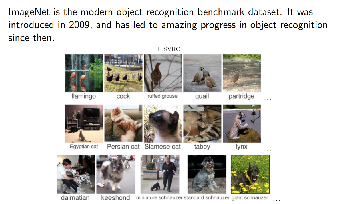
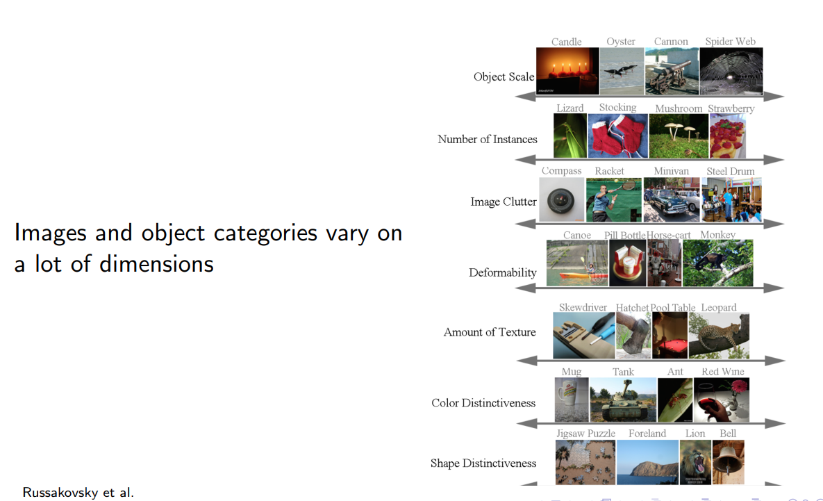
ImageNet I

ImageNet II

Used for: The ImageNet Large Scale Visual Recognition Challenge (ILSVRC), an annual benchmark competition for object recognition algorithms

Design Decisions

• Categories: Taken from a lexical database called WordNet
  • WordNet consists of “synsets”
  • Almost 22,000 classes used
  • The 1,000 most common chosen for the ILSVRC
  • The categories are really specific, e.g., hundreds of kinds of dogs

ImageNet III

• Size: 1.2 million full-sized images for the ILSVRC

• Source: Results from image search engines, hand-labeled by Mechanical Turkers

  • Labeling such specific categories was challenging; annotators had to be given the WordNet hierarchy, Wikipedia, etc.

• Normalization: None, although the contestants are free to do preprocessing

• Synsets are sets of synonymous words

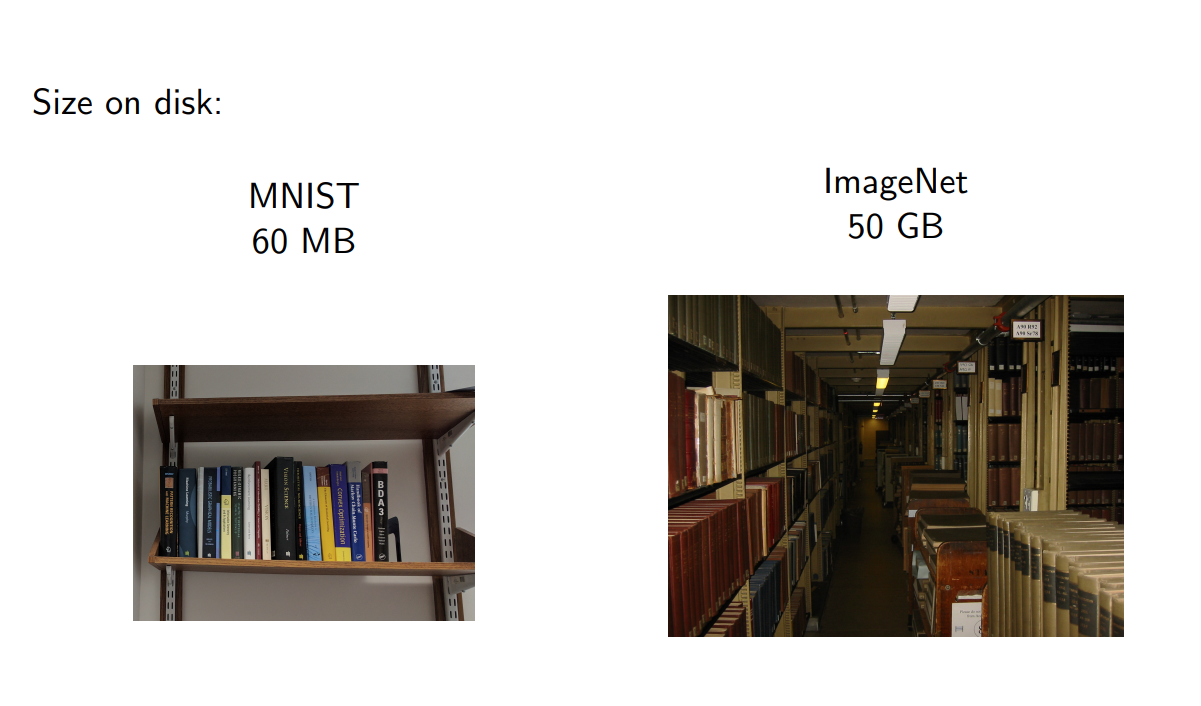
ImageNet IV

ImageNet V

ImageNet Results

Year	Model	Top-5 error
2010	Hand-designed descriptors + SVM	28.2%
2011	Compressed Fisher Vectors + SVM	25.8%
2012	AlexNet	16.4%
2013	a variant of AlexNet	11.7%
2014	GoogLeNet	6.6%
2015	deep residual nets	4.5%

• Top-5 error: True class among the 5 “best” results
• Human-performance is around 5.1%.
• ISVRC stopped running because the performance is already so good.

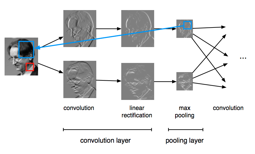
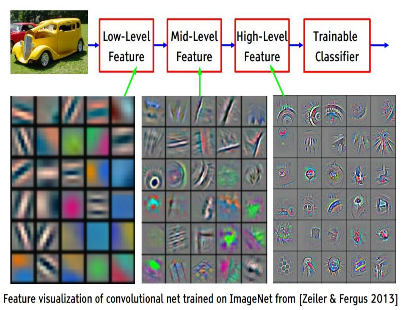
What features do CNN’s detect?

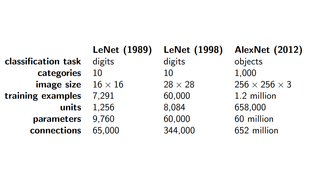
Size of a convnet

• Ways to measure the size of a network:
  • Number of units. The activations need to be stored in memory during training.
  • Number of weights. The weights need to be stored in memory / number of parameters determines overfitting.
  • Number of connections. There are approximately 3 add-multiply operations per connection (1 for the forward pass, 2 for the backward pass).
• Fully connected layer with \(M\) inputs and \(N\) outputs has \(MN\) connections / weights.

• The story for conv nets is more complicated.

Size of a convnet II

• Output Units: We assume no change in dimensions. For conv nets, this requires padding.
• Weights Much fewer weights because \(K^2 \ll W^2H^2\).
• Connections Not the same as weights anymore.

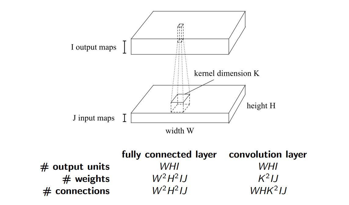
Size of a convnet III

LeNet Atchitecture

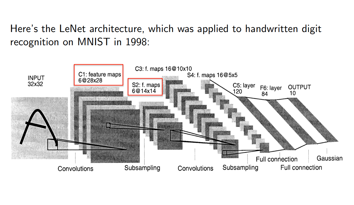
LeNet Architecture II

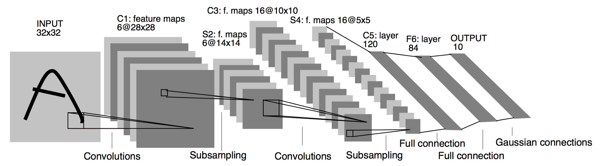
• Input: 32x32 pixel, greyscale image
• First convolution has 6 output features (5x5 convolution?)
• First subsampling is probably a max-pooling operation
• Second convolution has 16 output features (5x5 convolution?)
• …
• Some number of fully-connected layers at the end

ResNet Architecture

ResNet Architecture II

• Suppose we add another layer. How can we ensure that the new set of represented functions contains the old set, before the layer was added?
• Why do we need this? We’d like to get larger (nested) sets of functions as we add more layers and not just different (non-nested) sets.

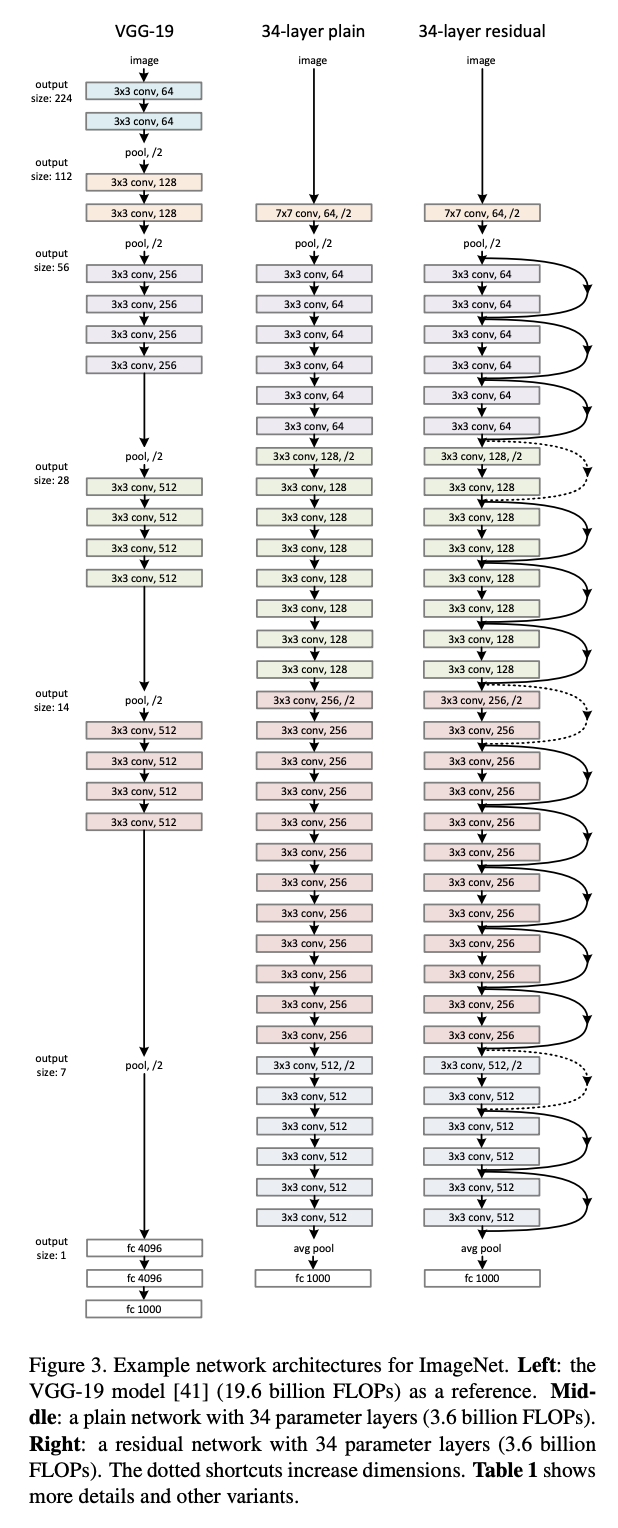
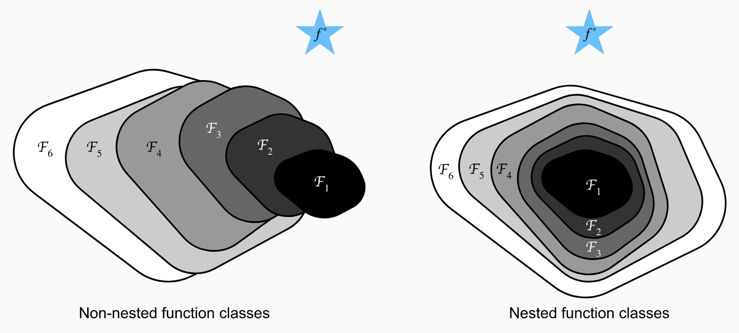
ResNet Blocks

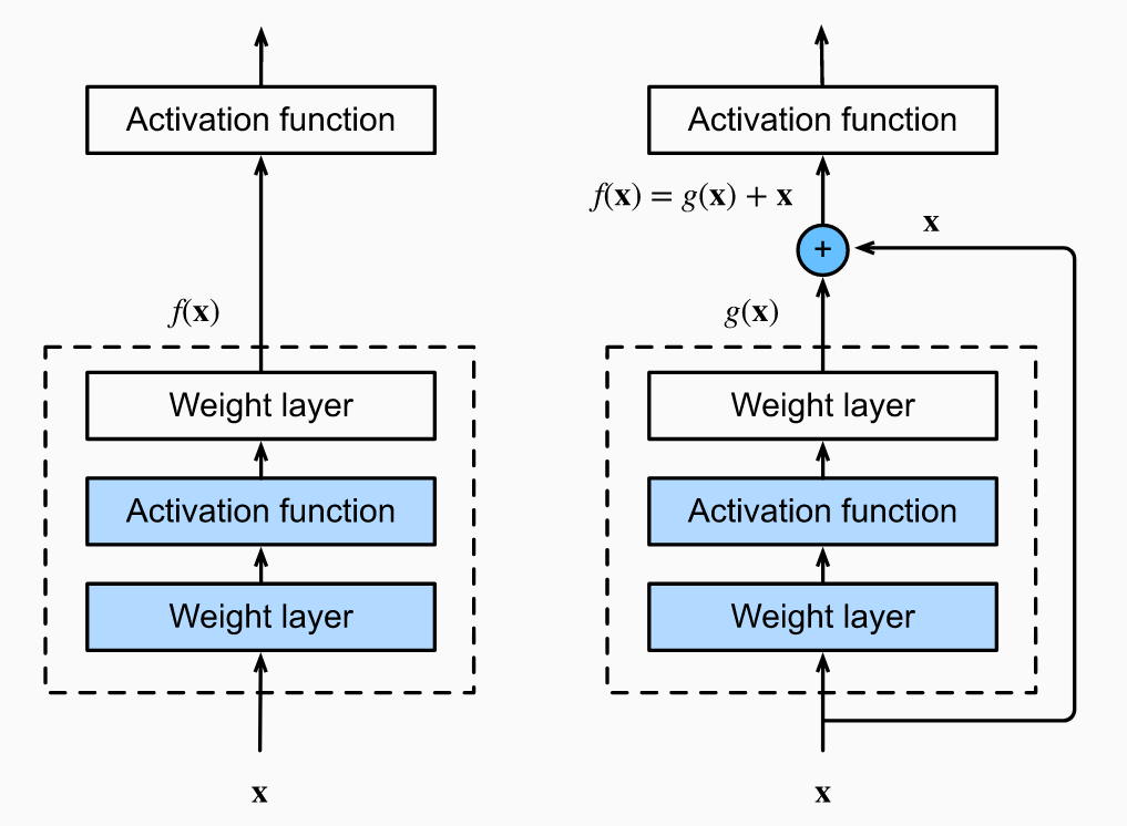
• Side effect of adding identity \(f(x) = x + g(x)\): better gradient propagation
• See https://d2l.ai/chapter_convolutional-modern/resnet.html

DenseNet Blocks

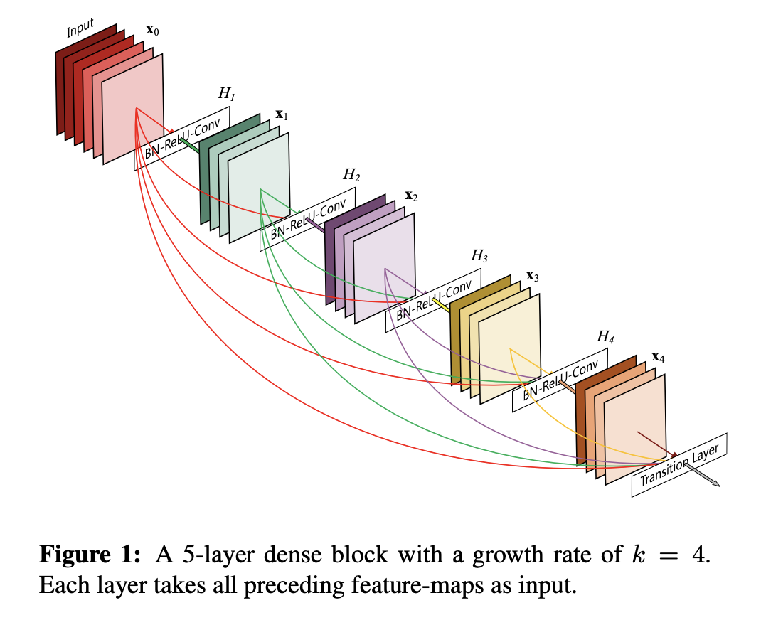
Same idea as ResNet blocks, but instead of addition \(f(x) = x + g(x)\) they use concatenation \(f(x) = [x, g(x)]\).

DenseNet Architecture

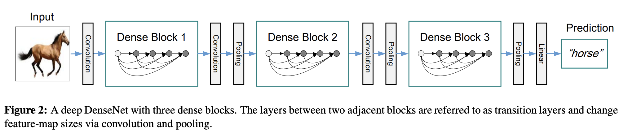
See https://d2l.ai/chapter_convolutional-modern/densenet.html

Wrap Up

Summary

• Computer Vision has been the main motivation for Conv Nets
• They draw inspiration from biological vision systems
• Key ideas are: local connectivity and weight sharing
• Conv Nets can be trained using backpropagation