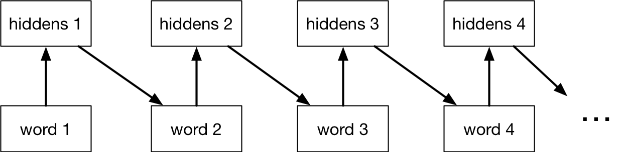
This means the model is memoryless, so it can only use information from its immediate context.
Recurrent Neural Network
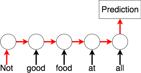
But sometimes long-distance context can be important.
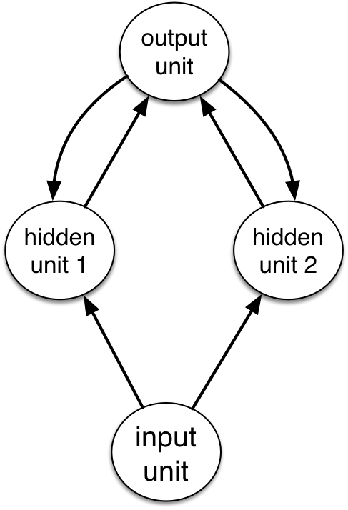
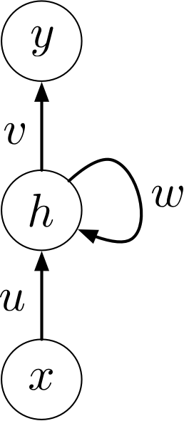
If we add connections between the hidden units, it becomes a recurrent neural network (RNN).
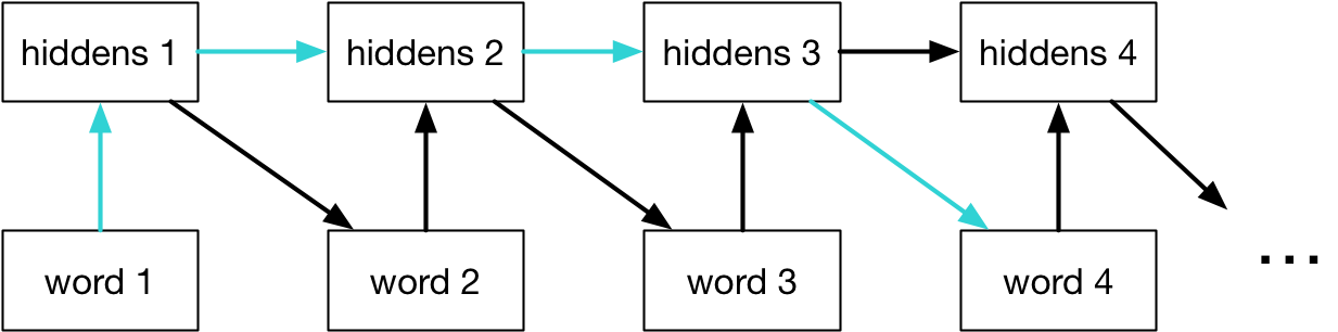
Having a memory lets an RNN use longer-term dependencies:
RNN Diagram
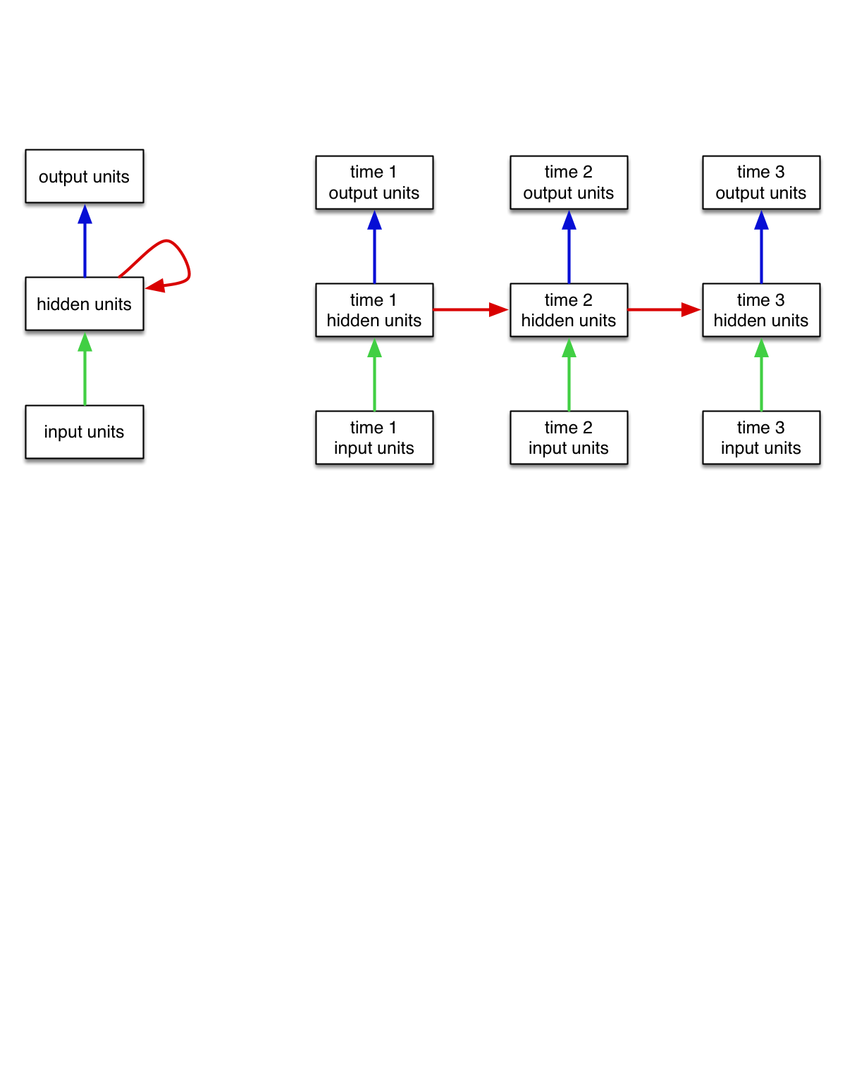
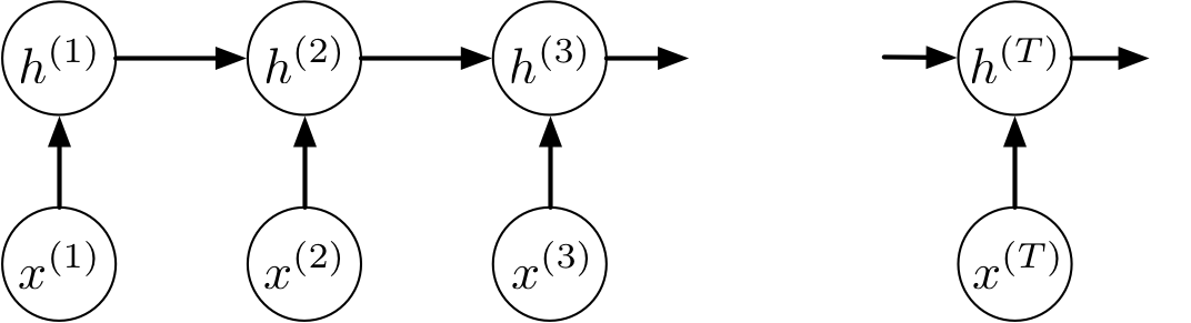
We can think of an RNN as a dynamical system with one set of hidden units which feed into themselves. The network’s graph would then have self-loops.
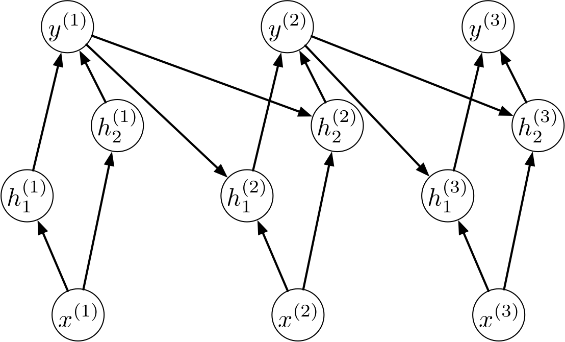
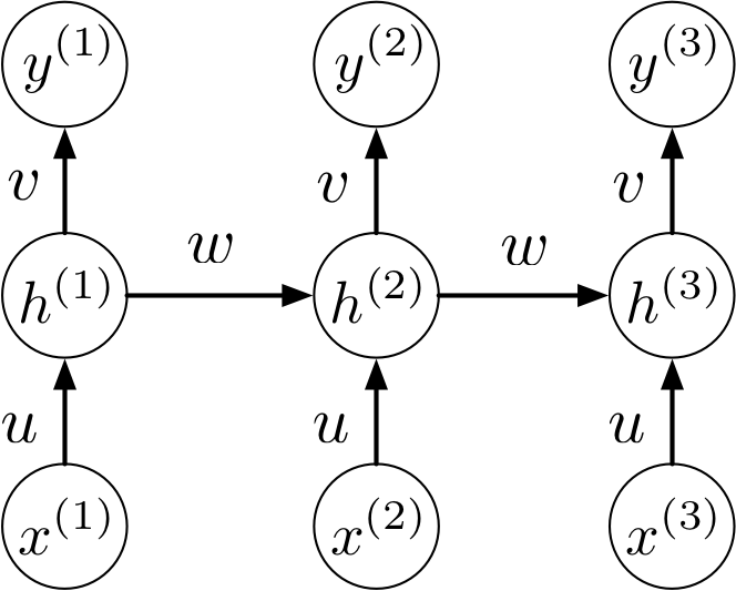
We can unroll the RNN’s graph by explicitly representing the units at all time steps. The weights and biases are shared between all time steps
Simple RNNs
Let’s go through a few examples of very simple RNNs to understand how RNNs compute predictions.
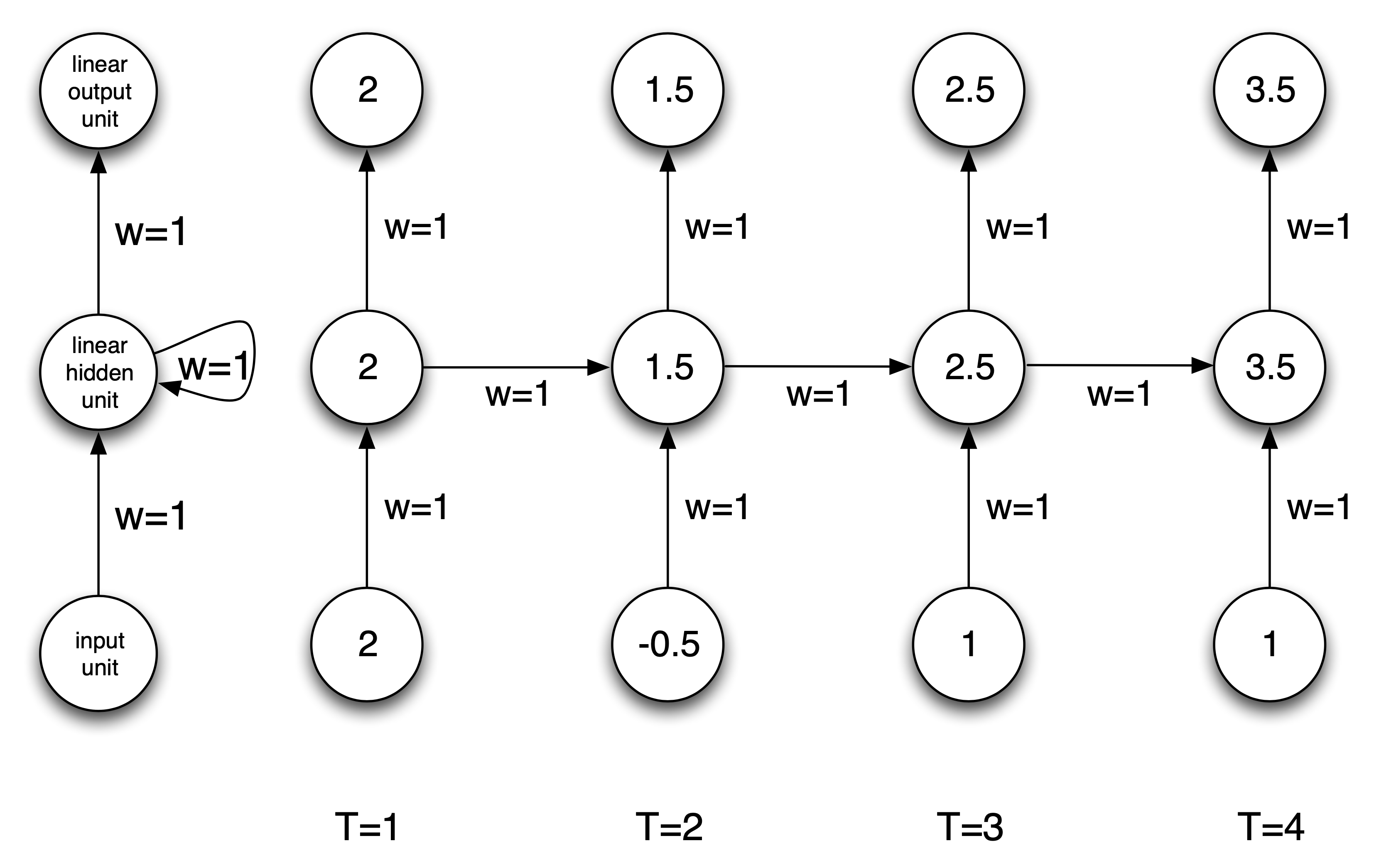
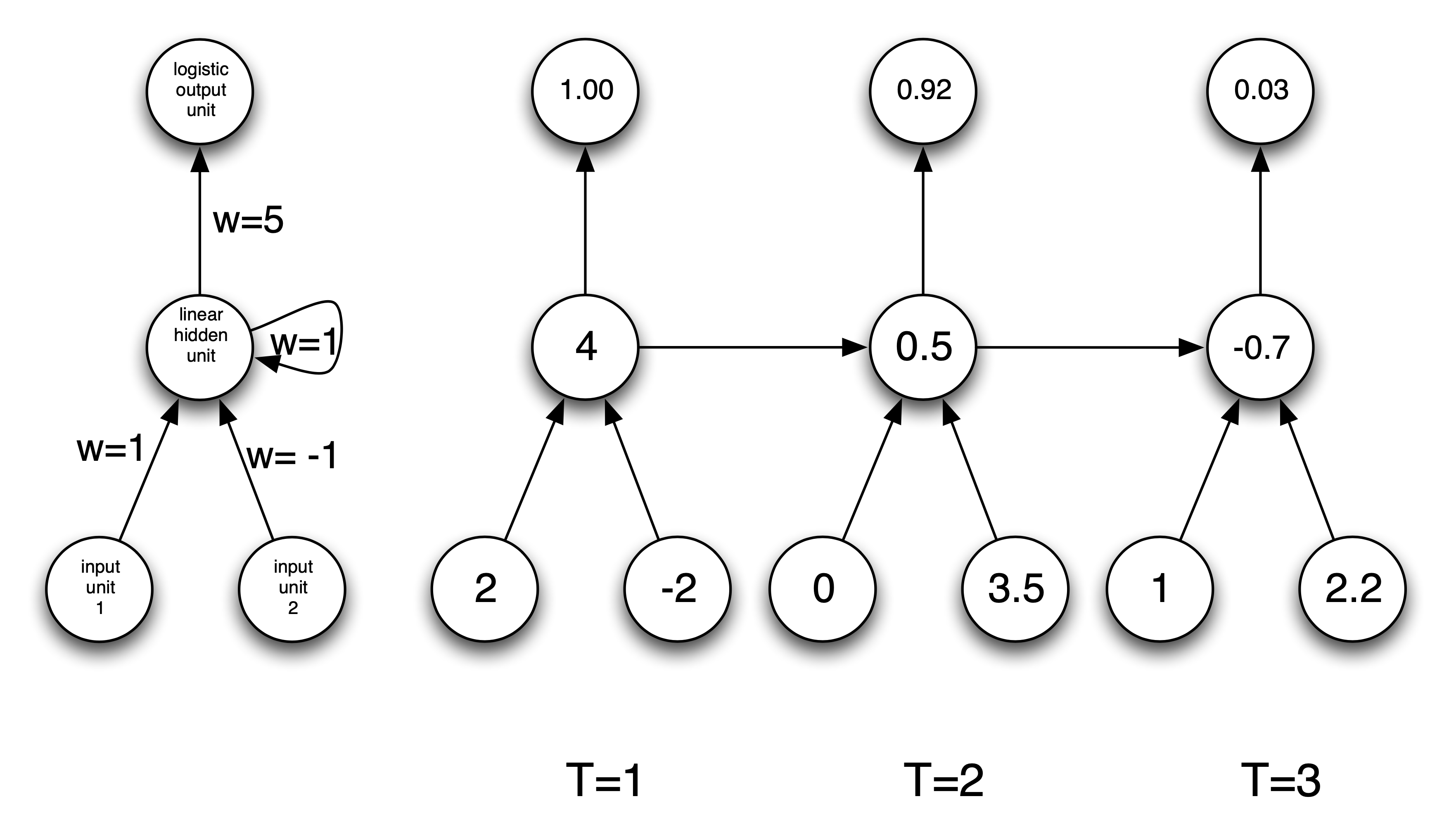
Simple RNN Example: Sum
This simple RNN takes a sequence of numbers as input (scalars), and sums its inputs.
Simple RNN Example 2: Comparison
This RNN takes a sequence of pairs of numbers as input, and determines if the total values of the first or second input are larger:
Simple RNN Example 3: Parity
Assume we have a sequence of binary inputs. We’ll consider how to determine the parity, i.e. whether the number of 1’s is even or odd. We can compute parity incrementally by keeping track of the parity of the input so far:
Parity bits:
Input:
0 1 1 0 1 1
\(\longrightarrow\)
0 1 0 1 1 0 1 0 1 1
Each parity bit is the XOR of the input and the previous parity bit. Parity is a classic example of a problem that’s hard to solve with a shallow feed-forward net, but easy to solve with an RNN.
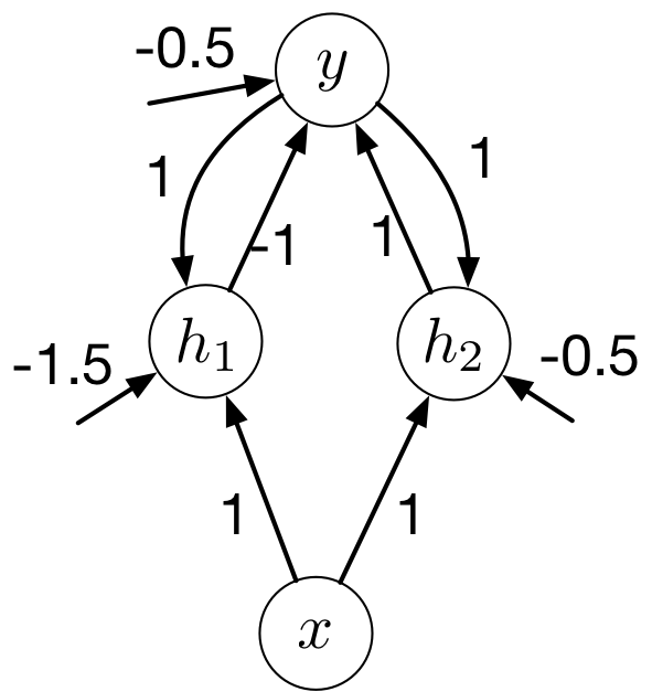
Parity Approach
Let’s find weights and biases for the RNN on the right so that it computes the parity. All hidden and output units are binary threshold units (\(h(x) = 1\) if \(x > 0\) and \(h(x) = 0\) otherise).
Strategy
The output unit tracks the current parity, which is the XOR of the current input and previous output.
The hidden units help us compute the XOR.
Parity Approach II
Unrolling Parity RNN
Parity Computation
The output unit should compute the XOR of the current input and previous output:
\(y^{(t-1)}\)
\(x^{(t)}\)
\(y^{(t)}\)
0
0
0
0
1
1
1
0
1
1
1
0
Computing Parity
Let’s use hidden units to help us compute XOR.
Have one unit compute AND, and the other one compute OR.
Then we can pick weights and biases just like we did for multilayer perceptrons.
Computing Parity II
\(y^{(t-1)}\)
\(x^{(t)}\)
\(h_1^{(t)}\)
\(h_2^{(t)}\)
\(y^{(t)}\)
0
0
0
0
0
0
1
0
1
1
1
0
0
1
1
1
1
1
1
0
Back Propagation Through Time
As you can guess, we don’t usually set RNN weights by hand. Instead, we learn them using backprop.
In particular, we do backprop on the unrolled network. This is known as backprop through time.
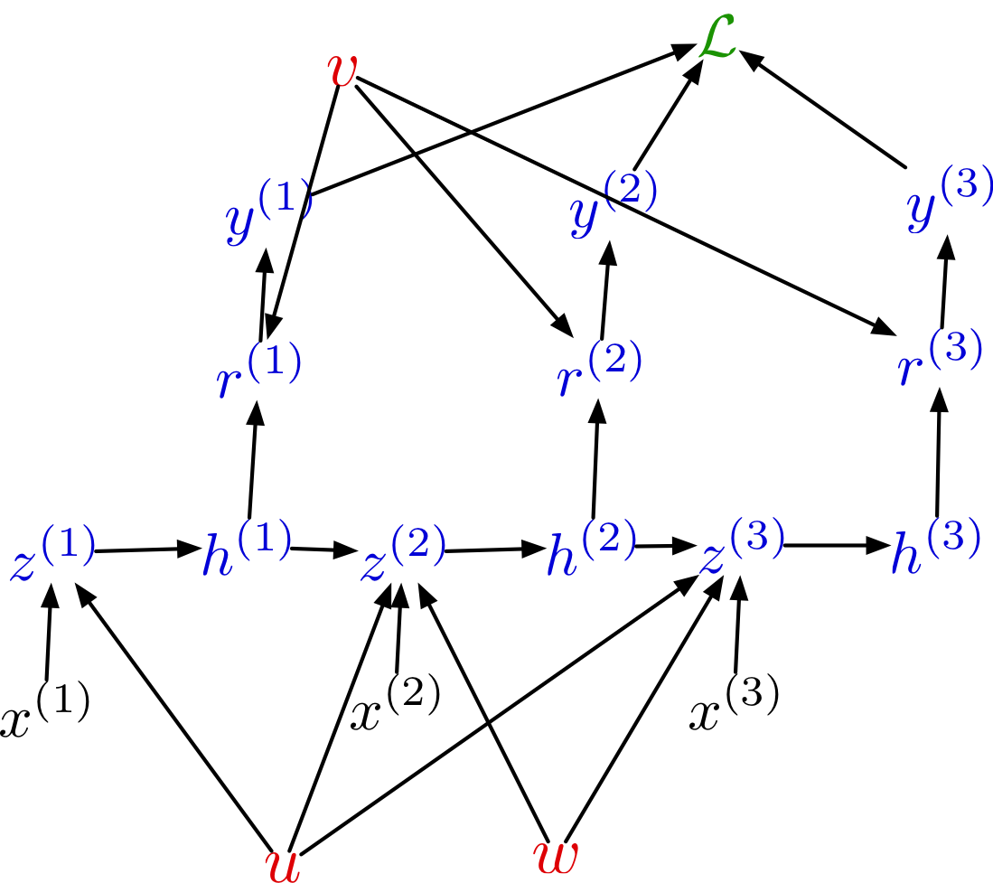
Unrolled BPTT
Here’s the unrolled computation graph. Notice the weight sharing.
What can RNNs compute?
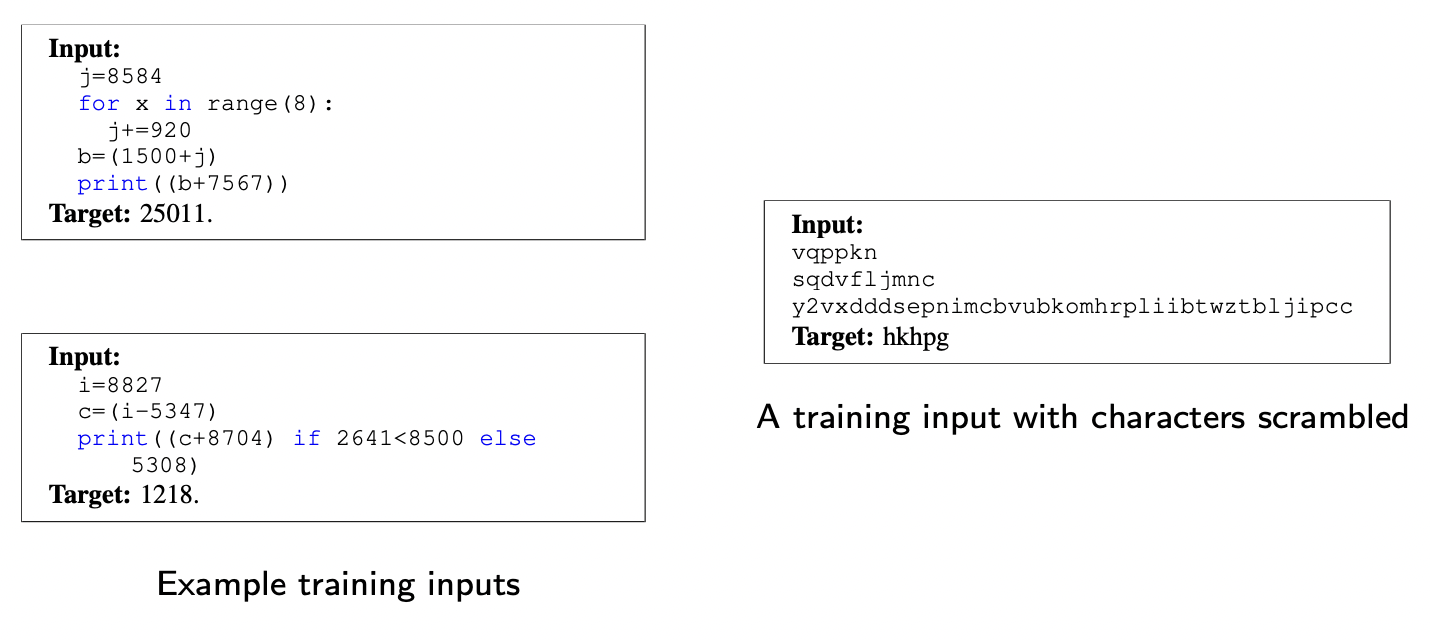
In 2014, Google researchers built an encoder-decoder RNN that learns to execute simple Python programs, one character at a time! https://arxiv.org/abs/1410.4615
What can RNNs compute?
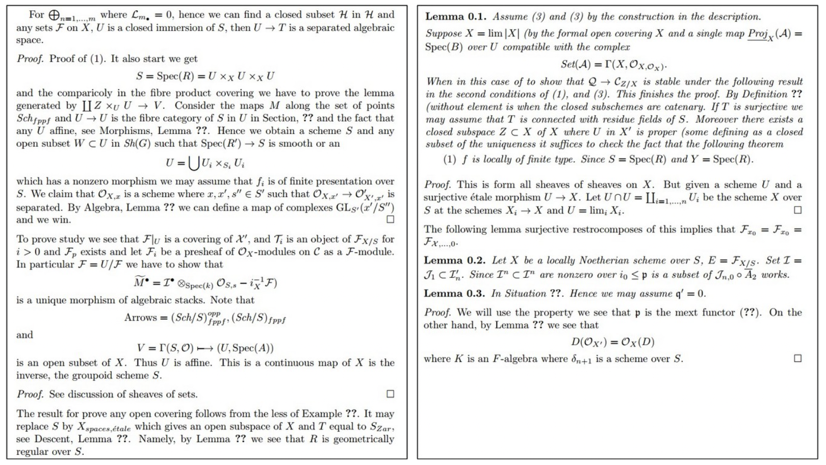
RNNs are good at learning complex syntactic structures: generate Algebraic Geometry LaTex source files that almost compiles:
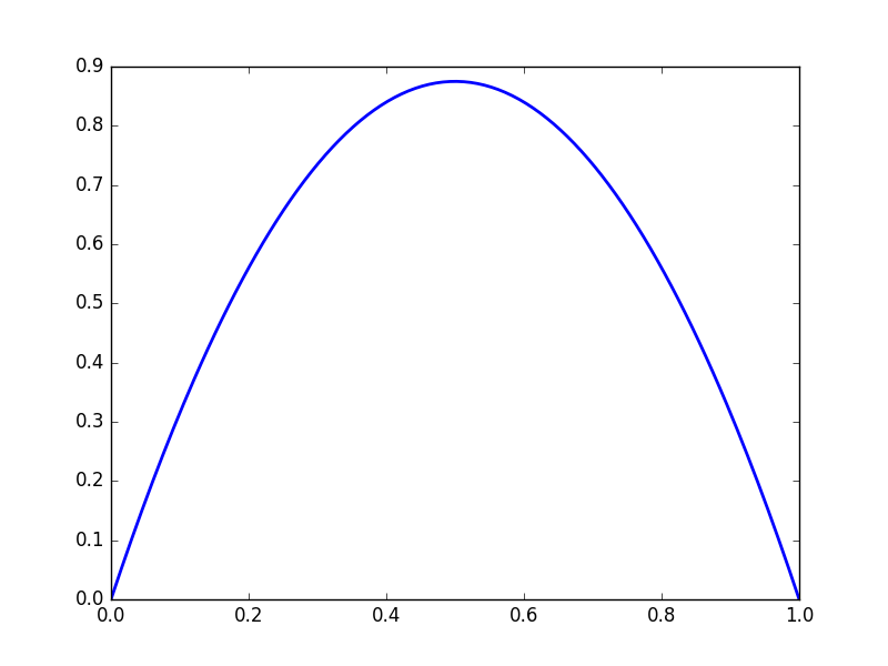
We get complicated behaviour from iterated functions. Consider \(f(x) = 3.5x(1-x)\)
\(y = f(x)\)
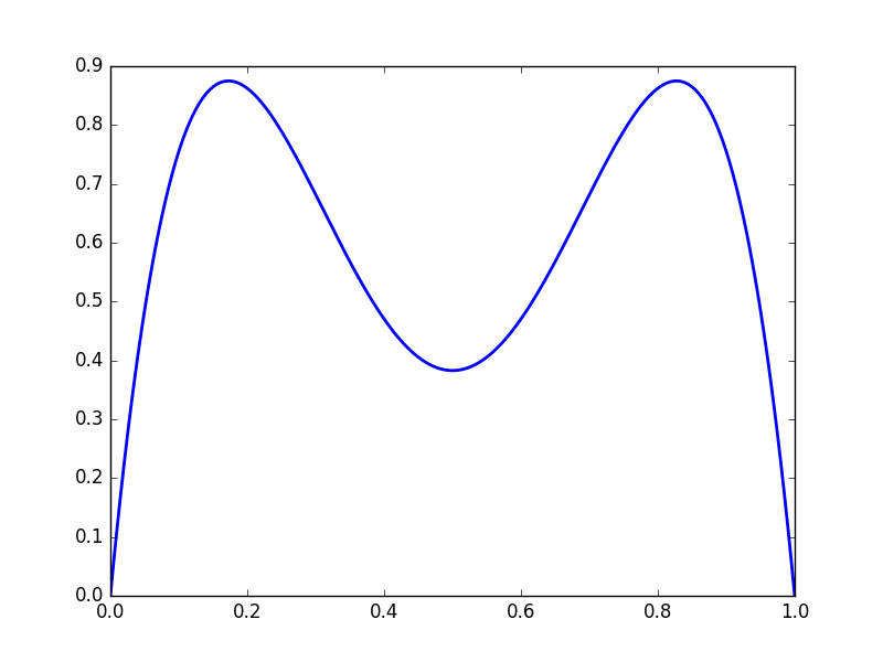
\(y = f(f(x))\)
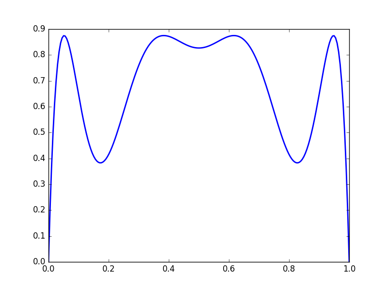
\(y = f^{\circ 3}(x)\)
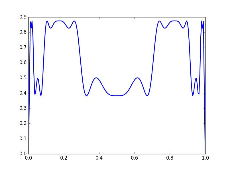
\(y = f^{\circ 6}(x)\)
Note that the function values gravitate towards fixed points, and that the derivatives becomes either very large or very small.
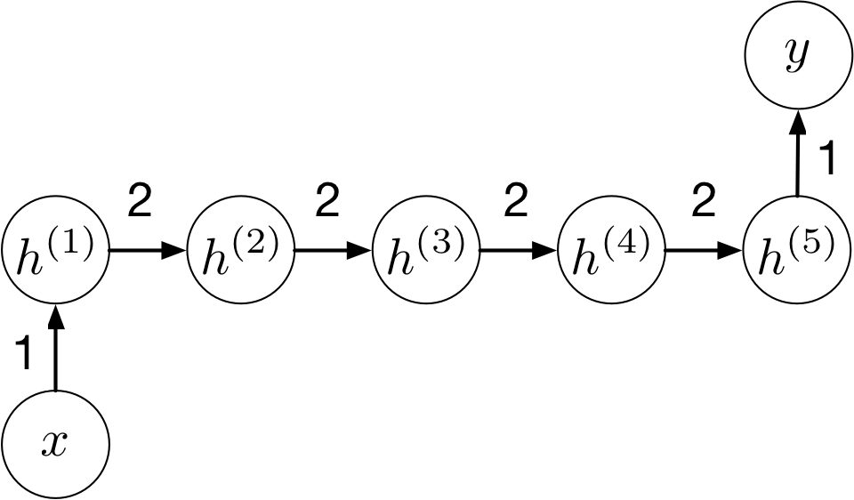
RNN with tanh activation
More concretely, consider an RNN with a tanh activation function:
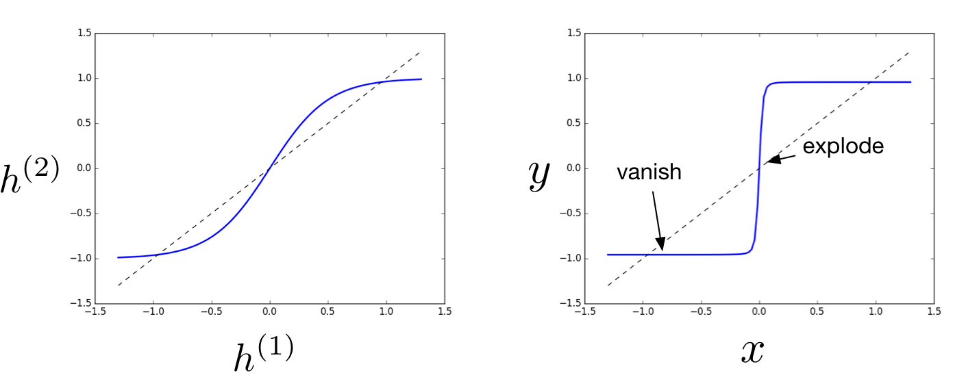
RNN with tanh activation II
The function computed by the network:
Cliffs
Repeatedly applying a function adds a new type possible loss landscape: cliffs, where the gradient of the loss with respect to a parameter is either close to 0, or very large.
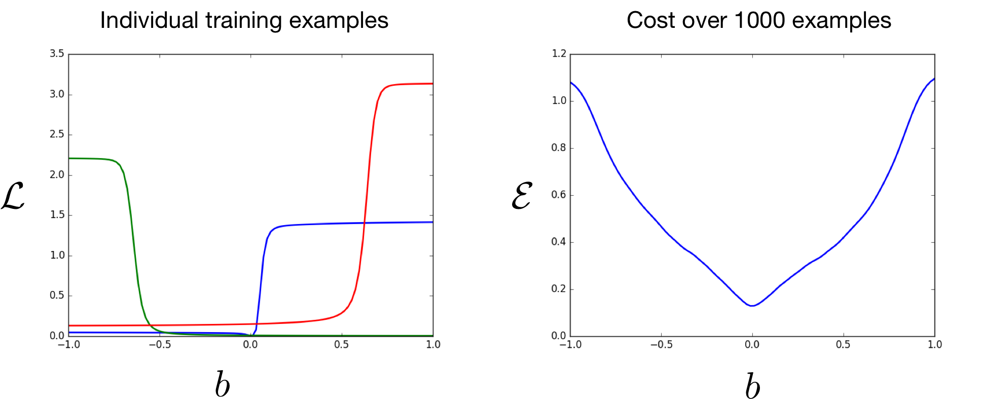
Cliffs II
Generally, the gradient will explode on some inputs and vanish on others. In expectation, the cost may be fairly smooth.
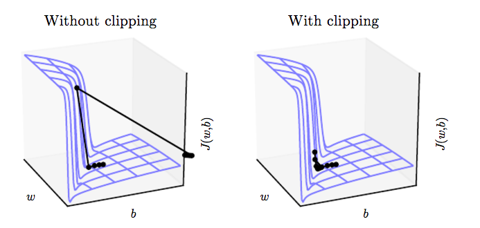
Gradient Clipping
One solution is to “clip” the gradient so that it has a norm of at most \(\eta\). Otherwise, update the gradient \({\bf g}\) with \({\bf g} \leftarrow \eta\frac{{\bf g}}{||{\bf g}||}\)
The gradients are biased, but at least they don’t blow up:
Gradient clipping solves the exploding gradient problem, but not the vanishing gradient problem.
Learning Long-Term Dependencies
Idea: Initialization
Hidden units are a kind of memory. Their default behaviour should be to keep their previous value.
If the function \({\bf h}^{(t)} = f({\bf h}^{(t-1)}, {\bf x}^{(t)})\) is close to the identity, then the gradient computations \(\displaystyle \frac{\partial {\bf h}^{(t)}}{\partial {\bf h}^{(t-1)}}\) are stable.
This initialization allows learning much longer-term dependencies than “vanilla” RNNs
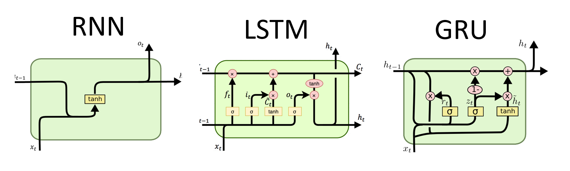
Long-Term Short Term Memory
Change the architecture of the recurrent neural network by replacing each single unit in an RNN by a “memory block”:
LSTM
LSTM Math
In each step, we have a vector of memory cells \({\bf c}\), a vector of hidden units \({\bf h}\) and vectors of input, output, and forget gates \({\bf i}\), \({\bf o}\), and \({\bf f}\).
There’s a full set of connections from all the inputs and hiddens to the inputs and all of the gates:
Exercise: show that if \({\bf f}_{t+1} = 1\), \({\bf i}_{t+1} = 0\), and \({\bf o}_{t} = 0\), then the gradient of the memory cell gets passed through unmodified, i.e., \(\bar{{\bf c}_t} = \bar{{\bf c}_{t+1}}\).
Key Takeaways
You should be able to understand…
why learning long-term dependencies is hard for vanilla RNNs
why gradients vanish/explode in a vanilla RNN
what cliffs are and how repeated application of a function generates cliffs
what gradient clipping is and when it is useful
the mathematics behind why gating works
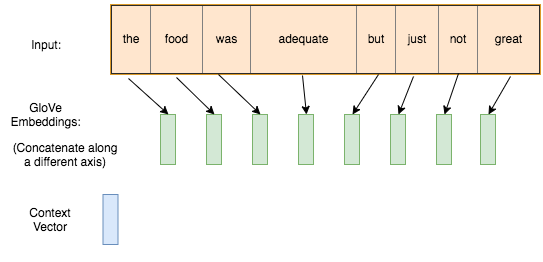
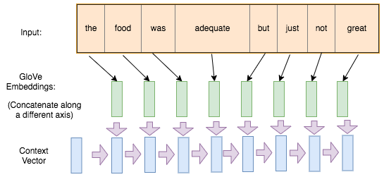
Text Generation with RNN
RNN Hidden States
RNN For Prediction:
Process tokens one at a time
Hidden state is a representation of all the tokens read thus far
RNN For Generation:
Generate tokens one at a time
Hidden state is a representation of all the tokens to be generated
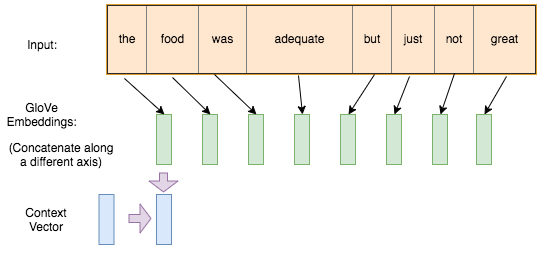
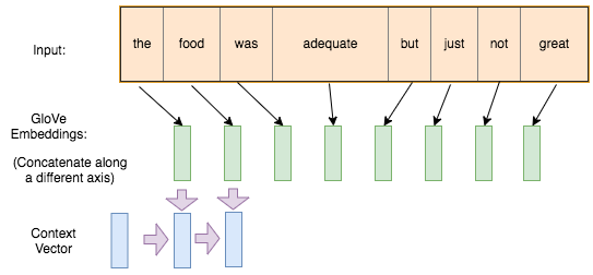
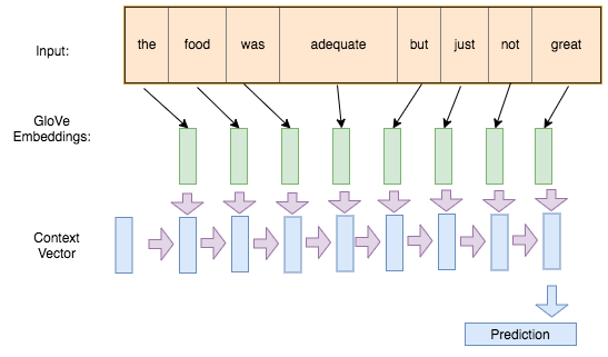
RNN Hidden State Updates
RNN for Prediction:
Update hidden state with new input (token)
Get prediction (e.g. distribution over possible labels)
RNN for Generation:
Get prediction distribution of next token
Generate a token from the distribution
Update the hidden state with new token
Text Generation Diagram
Get prediction distribution of next token
Generate a token from the distribution
Update the hidden state with new token
Test Time Behaviour of Generative RNN
Unlike other models we discussed so far, the training time behaviour of Generative RNNs will be different from the test time behaviour
Test time behaviour at each time step:
Obtain a distribution over possible next tokens
Sample a token from that distribution
Update the hidden state based on the sample token
Training Time Behaviour of Generative RNN
During training, we try to get the RNN to generate one particular sequence in the training set. At each time step:
Obtain a distribution over possible next tokens
Compare this with the actual next token
Q1: What kind of a problem is this? (regression or classification?)
Q2: What loss function should we use during training?
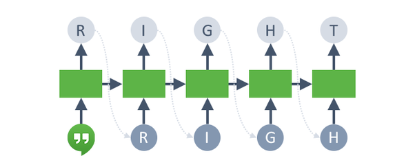
Text Generation: First Step
Start with an initial hidden state
Update the hidden state with a “<BOS>” (beginning of string) token to initiate the hidden state
Get the distribution over the first character
Compute the cross-entropy loss against the ground truth (R)
Text Generation with Teacher Forcing
Update the hidden state with the ground truth token (R) regardless of the prediction from the previous step
This technique is called teaching forcing
Get the distribution over the second character
Compute the cross-entropy loss against the ground truth (I)
Text Generation: Later Steps
Continue until we get to the “<EOS>” (end of string) token
Some Remaining Challenges
Vocabularies can be very large once you include people, places, etc.
It’s computationally difficult to predict distributions over millions of words.
How do we deal with words we haven’t seen before?
In some languages, it’s hard to define what should be considered a word.
Character vs Word-level
Another approach is to model text one character at a time
This solves the problem of what to do about previously unseen words.
Note that long-term memory is essential at the character level!
Sequence-to-Sequence Architecture
Neural Machine Translation
Say we want to translate, e.g. English to French sentences.
We have pairs of translated sentences to train on.
Here, both the inputs and outputs are sequences!
What can we do?
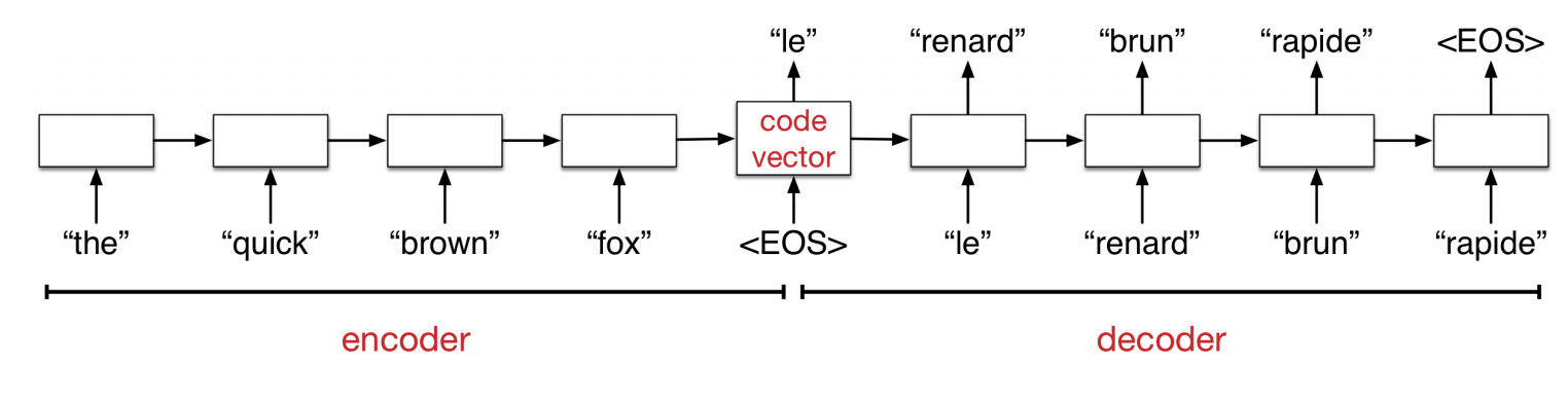
Sequence-to-sequence architecture
The network first reads and memorizes the sentences.
When it sees the “end token”, it starts outputting the translation.
The “encoder” and “decoder” are two different networks with different weights.
Wrap Up
Summary
Recurrent Neural Networks can be used for learning sequence data
Training RNNs may suffer from gradient explosion and vanishing
Important Applications of RNNs are text generation and sequence to sequence modelling