CSC413 Neural Networks and Deep Learning

Lecture 12

Announcements

• Book a meeting to discuss your project with an instructor if you haven’t already!

• You should have an overfit version of the model already

• This is your first step, and should let you know the time/memory requirements of your model

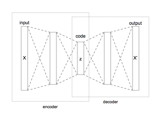
Review: Autoencoders

A couple of weeks ago, we discussed the autoencoders

• Encoder: maps \(x\) to a low-dimensional embedding \(z\)

• Decoder: uses the low-dimensional embedding \(z\) to reconstructs \(x\)

Let’s see how much you remember!

Review Q1

What was the objective that we used to train the autoencoder?

Review Q2

If we train an autoencoder, what tasks can we accomplish with just the encoder portion of the autoencoder?

Review Q3

If we train an autoencoder, what tasks can we accomplish with mainly the decoder portion of the autoencoder?

Review Q4

What are some limitations of the autoencoder?

Autoencoder Limitations

• Images are blurry due to the use of MSE loss

• It’s not certain what good values of embeddings \(z\) would be
  • Which part of the embedding space does the encoder maps data to?
  • This uncertainty means that we can’t generate images without referring back to the encoder

• It’s not clear what the dimension of the embedding \(z\) should be

Autoencoder Limitations II

Could we resolve (but not all) some of the issues with autoencoder, if we use a more theoretically grounded approach?

Is there a probabilistic version of the autoencoder model?

Variational Autoencoders

Generative Model

In CSC311, we learned about generative models that describe the distribution that the data comes from

• i.e. describe the distribution \({\bf x} \sim p({\bf x})\), where \({\bf x}\) is a single data point

For example, in the Naive Bayes model for data \({\bf x}\) (e.g. bag-of-word encoding of an email, which could be spam or not spam) with \({\bf x} \sim p({\bf x})\), we assumed that \(p({\bf x}) = \sum_c p({\bf x}|c)p(c)\), where \(c\) is either spam or not spam. We made further assumptions about \(p({\bf x}|c)\), e.g. that each \(x_i\) is an independent Bernoulli.

Mathematical Notation and Assumptions

Data \(x_i \in \mathbb{R}^d\) are:

• independent, identically distributed (i.i.d)

• generated from the following joint distribution (with the true parameter \(\theta^{*}\) unknown)

\[p_{\theta^{*}}(\textbf{z}, \textbf{x}) = p_{\theta^{*}}(\textbf{z})p_{\theta^{*}}(\textbf{x} | \textbf{z})\]

Where \({\bf z}\) is a low-dimensional vector (latent embedding)

Mathematical Notation and Assumptions II

• Example \({\bf x}\) could be an MNIST digit

• Think of \({\bf z}\) as encoding digit features like digit shape, tilt, line thickness, font style, etc…

• To generate an image, we first sample from the prior distribution \(p_{\theta^{*}}(\textbf{z})\) to decide on these digit features, and use \(p_{\theta^{*}}(\textbf{x} | \textbf{z})\) to generate an image given those features

Intractability

Our data set is large, and so the following are intractable

• evidence \(p_{\theta^{*}}(\textbf{x})\)

• posterior distributions \(p_{\theta^{*}}(\textbf{z} | \textbf{x})\)

In other words, exactly computing the distribution of \(p(\textbf{x})\) and \(p(\textbf{z} | \textbf{x})\) using our dataset has high runtime complexity.

The Decoder and Encoder

With this assumption, we can think of the autoencoder as doing the following:

Decoder: A point approximation of the true distribution \(p_{\theta^{*}}(\textbf{x}|\textbf{z})\)

Encoder: Making a point prediction for the value of the latent vector \(z\) that generated the image \(x\)

The Decoder and Encoder II

Alternative:

• what if, instead, we try to infer the distribution \(p_{\theta^{*}}(\textbf{z}|\textbf{x})\)?

VAE Setup so far

Decoder: An approximation of the true distribution \(p_{\theta^{*}}(\textbf{x}|\textbf{z})\)

Encoder: An approximation of the true distribution \(p_{\theta^{*}}(\textbf{z}|\textbf{x})\)

Computing the encoding distribution \(p_{\theta^{*}}(\textbf{z}|\textbf{x})\)

Unfortunately, the true distribution \(p_{\theta^{*}}({\bf z}|{\bf x})\) is complex (e.g. can be multi-modal).

But can we approximate this distribution with a simpler distribution?

Let’s restrict our estimate \(q_\phi({\bf z}|{\bf x}) = \mathcal{N}({\bf z}; \boldsymbol{\mu}, \boldsymbol{\Sigma})\) to be a multivariate Gaussian distribution with \(\phi = (\boldsymbol{\mu}, \boldsymbol{\Sigma})\)

Computing the encoding distribution \(p_{\theta^{*}}(\textbf{z}|\textbf{x})\) II

• It suffices to estimate the mean \(\boldsymbol{\mu}\) and covariance matrix \(\boldsymbol{\Sigma}\) of \(q_\phi({\bf z}|{\bf x})\)
• Let’s make it simpler and assume that the covariance matrix is diagonal, \(\boldsymbol{\Sigma}=\sigma^2 \textbf{I}_{d \times d}\)

(Note: we don’t have to make this assumption, but it will make computation easier later on)

VAE Setup so far

Decoder: An approximation of the true distribution \(p_{\theta^{*}}(\textbf{x}|\textbf{z})\)

Encoder: Predicts the mean and standard deviations of a distribution \(q_\phi({\bf z}|{\bf x})\), so that the distribution is close to the true distribution \(p_{\theta^{*}}(\textbf{z}|\textbf{x})\)

We want our estimate distribution to be close to the true distribution. How do we measure the difference between distributions?

(Discrete) Entropy

\[H[X] = \sum_x p(X = x) \log \left(\frac{1}{p(X = x)}\right) = \text{E}\left[\log \frac{1}{p(X)}\right]\]

Many ways to think about this quantity:

• The expected number of yes/no questions you would need to ask to correctly predict the next symbol sampled from distribution \(p(X)\)

(Discrete) Entropy II

• The expected “surprise” or “information” in the possible outcomes of random variable \(X\)

• The minimum number of bits required to compress a symbol \(x\) sampled from distribution \(p(X)\)

(Discrete) Entropy of a Coin Flip

• Entropy of a fair coin flip is \(0.5\log(2) + 0.5\log(2) = \log(2) = 1\) bits
• Entropy of a fair dice is \(\log(6) = 2.58\) bits

• Entropy of characters in English words is about 2.62 bits

• Entropy of characters from the English alphabet selected uniformly at random is \(\log(26) = 4.7\) bits

Kullback-Leibler Divergence

Also called: KL Divergence, Relative Entropy

For discrete probability distributions:

\[D_\text{KL}(q(z) ~||~ p(z)) = \sum_z q(z) \log \left(\frac{q(z)}{p(z)}\right)\]

For continuous probability distributions:

\[D_\text{KL}(q(z) ~||~ p(z)) = \int q(z) \log \left(\frac{q(z)}{p(z)}\right)\, dz\]

KL Divergence Example Computation

Approximating an unfair coin with a fair coin.

• \(p(z = 1) = 0.7\) and \(p(z = 0) = 0.3\)

• \(q(z = 1) = q(z = 0) = 0.5\)

KL Divergence Example Computation II

\[\begin{align*} D_\text{KL}(q(z) ~||~ p(z)) &= \sum_z q(z) \log \left(\frac{q(z)}{p(z)}\right) \\ &= q(0) \log \left(\frac{q(0)}{p(0)}\right) + q(1) \log \left(\frac{q(1)}{p(1)}\right) \\ &= 0.5 \log \left(\frac{0.5}{0.3}\right) + 0.5 \log \left(\frac{0.5}{0.7}\right) \\ &= 0.872 \end{align*}\]

KL Divergence is not Symmetric!

Approximating a fair coin with an unfair coin.

• \(p(z = 1) = 0.7\) and \(p(z = 0) = 0.3\)

• \(q(z = 1) = q(z = 0) = 0.5\)

KL Divergence is not Symmetric! II

\[\begin{align*} D_\text{KL}(p(z) ~||~ q(z)) &= \sum_z p(z) \log \left(\frac{p(z)}{q(z)}\right) \\ &= p(0) \log \left(\frac{p(0)}{q(0)}\right) + p(1) \log \left(\frac{p(1)}{q(1)}\right) \\ &= 0.3 \log \left(\frac{0.3}{0.5}\right) + 0.7 \log \left(\frac{0.7}{0.5}\right) \\ &= 0.823 \\ &\neq D_\text{KL}(q(z) ~||~ p(z)) \end{align*}\]

Minimizing KL Divergence

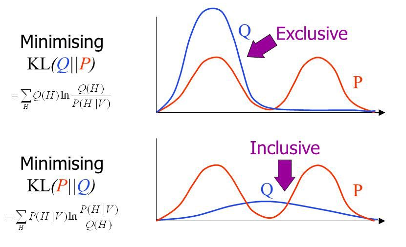
KL Divergence Properties

The KL divergence is a measure of the difference between probability distributions.

KL divergence is an asymmetric, nonnegative measure, not a norm. It doesn’t obey the triangle inequality.

KL divergence is always positive. Hint: you can show this using the inequality \(\ln(x) \leq x - 1\) for \(x > 0\).

KL Divergence: Continuous Example

Suppose we have two Gaussian distributions \(p(x) \sim N\left(\mu_1, \sigma_1^2\right)\) and \(q(x) \sim N\left(\mu_2, \sigma_2^2\right)\).

What is the KL divergence \(D_\text{KL}(p(z) ~||~ q(z))\)?

Recall:

\[p\left(z; \mu_1, \sigma_1^2\right) = \frac{1}{\sqrt{2 \pi \sigma_1^2}} e^{-\frac{(z - \mu_1)^2}{2\sigma_1^2}}\]

\[\log \left(p\left(z; \mu_1, \sigma_1^2\right)\right) = - \log \sqrt{2 \pi \sigma_1^2} - \frac{(z - \mu_1)^2}{2\sigma_1^2}\]

KL Divergence: Entropy and Cross-Entropy

We can split the KL divergence into two terms, which we can compute separately:

\[\begin{align*} D_\text{KL}(p(z) ~||~ q(z)) &= \int p(z) \log \frac{p(z)}{q(z)} dz \\ &= \int p(z) (\log p(z) - \log q(z)) dz \\ &= \int p(z) \log p(z) dz - \int p(z) \log q(z) dz \\ &= -\text{entropy} - \text{cross-entropy} \end{align*}\]

KL Divergence: Continuous Example, Entropy Computation

\[\begin{align*} \int p(z) \log\left(p(z)\right)\, dz \\ &\hspace{-24pt}= \int p(z) \left(-\log\left(\sqrt{2 \pi \sigma_1^2}\right) - \frac{(z - \mu_1)^2}{2\sigma_1^2}\right)\, dz \\ &\hspace{-24pt}= - \int p(z) \frac{1}{2}\log\left(2 \pi \sigma_1^2\right)\, dz - \int p(z) \frac{(z - \mu_1)^2}{2\sigma_1^2}\, dz \\ &\hspace{-24pt}= \ldots \end{align*}\]

KL Divergence: Continuous Example, Entropy Computation II

\[\begin{align*} \ldots &= -\frac{1}{2}\log\left(2 \pi \sigma_1^2\right) \int p(z)\, dz - \frac{1}{2\sigma_1^2}\int p(z) (z - \mu_1)^2\, dz \\ &= -\frac{1}{2}\log\left(2 \pi \sigma_1^2\right) - \frac{1}{2} \\ &= -\frac{1}{2}\log\left(\sigma_1^2\right) - \frac{1}{2}\log (2 \pi) - \frac{1}{2} \end{align*}\]

Since \(\displaystyle \int p(z)\, dz = 1\) and \(\displaystyle\int p(z) (z - \mu_1)^2\, dz = \sigma_1^2\)

KL Divergence: Continuous Example, Cross-Entropy Computation

\[\begin{align*} \int p(z) \log\left(q(z)\right)\, dz \\ &\hspace{-36pt}= \int p(z) \left(-\log\left(\sqrt{2 \pi \sigma_2^2}\right) - \frac{(z - \mu_2)^2}{2\sigma_2^2}\right)\, dz \\ &\hspace{-36pt}= -\int p(z) \frac{1}{2}\log (2 \pi \sigma_2^2)\, dz - \int p(z) \frac{(z - \mu_2)^2}{2\sigma_2^2}\, dz \\ &\hspace{-36pt}= -\frac{1}{2}\log (2 \pi \sigma_2^2) - \frac{1}{2\sigma_2^2}\int p(z) (z - \mu_2)^2\, dz = \ldots \end{align*}\]

KL Divergence: Continuous Example, Cross-Entropy Computation II

\[\ldots = - \frac{1}{2}\log (2 \pi \sigma_2^2) - \frac{\sigma_1^2 + (\mu_1-\mu_2)^2}{2\sigma_2^2}\]

Back to Autoencoders: Summary so far

Autoencoder:

• Decoder: point estimate of \(p_{\theta^{*}}(\textbf{x} | \textbf{z})\)

• Encoder: point estimate of the value of \(\textbf{z}\) that generated the image \(\textbf{x}\)

Back to Autoencoders: Summary so far II

VAE:

• Decoder: probabilistic estimate of \(p_{\theta^{*}}(\textbf{x} | \textbf{z})\)

• Encoder: probabilistic estimate of a Gaussian distribution \(q_{\phi}(\textbf{z} | \textbf{x})\) that approximates the distribution \(p_{\theta^{*}}(\textbf{z} | \textbf{x})\)
  • In particular, our encoder will be a neural network that predicts the mean and standard deviation of \(q_{\phi}(\textbf{z} | \textbf{x})\)
  • We can then sample \({\bf z}\) from this distribution!

VAE Objective

But how do we train a VAE?

We want to maximize the likelihood of our data:

\[\displaystyle \log(p(x)) = \log\left(\int p(x|z)p(x)\, dz\right)\]

And we want to make sure that the distributions \(q(z|x)\) and \(p(z|x)\) are close:

• We want to minimize \(D_\text{KL}(q({\bf z}|{\bf x}) ~||~ p({\bf z} | {\bf x}))\)

• This is a measure of encoder quality

VAE Objective II

In other words, we want to maximize

\[-D_\text{KL}(q({\bf z}|{\bf x}) ~||~ p({\bf z} | {\bf x})) + \log(p(x))\]

How can we optimize this quantity in a tractable way?

VAE: Evidence Lower-Bound

\[\begin{align*} D_\text{KL}(q({\bf z}|{\bf x}) ~||~ p({\bf z} | {\bf x})) &= \int q({\bf z}|{\bf x}) \log\left(\frac{q({\bf z}|{\bf x})}{p({\bf z}|{\bf x})}\right)\, dz \\ &= \text{E}_q\left(\log\left(\frac{q({\bf z}|{\bf x})}{p({\bf z}|{\bf x})}\right)\right) \\ &= \text{E}_q (\log (q({\bf z}|{\bf x}))) - \text{E}_q(\log(p({\bf z}|{\bf x}))) \\ &= \text{E}_q(\log(q({\bf z}|{\bf x}))) - \text{E}_q(\log(p({\bf z},{\bf x}))) \\ &\hspace{12pt} + \text{E}_q(\log(p({\bf x}))) \\ &= \text{E}_q(\log(q({\bf z}|{\bf x}))) - \text{E}_q(\log(p({\bf z},{\bf x}))) \\ &\hspace{12pt} + \log p({\bf x}) \end{align*}\]

VAE: Evidence Lower-Bound II

We’ll define the evidence lower-bound: \[\text{ELBO}_q({\bf x}) = \text{E}_q(\log(p({\bf z},{\bf x})) - \log(q({\bf z}|{\bf x})))\]

So we have \[\log(p({\bf x})) - D_\text{KL}(q({\bf z}|{\bf x}) ~||~ p({\bf z} | {\bf x})) = \text{ELBO}_q({\bf x})\]

Optimizing the ELBO

The ELBO gives us a way to estimate the gradients of \(\log(p({\bf x})) - D_\text{KL}(q({\bf z}|{\bf x}) ~||~ p({\bf z} | {\bf x}))\)

How?

\[\text{ELBO}_q({\bf x}) = \text{E}_q(\log(p({\bf z},{\bf x})) - \log(q({\bf z}|{\bf x})))\]

• The right hand side of this expression is an expectation over \(z \sim q(z|x)\)

• To estimate the ELBO, we can sample from the distribution \(z \sim q(z|x)\), and compute the terms inside.

Optimizing the ELBO II

• We can estimate gradients in the same way—this is called a Monte-Carlo gradient estimator

Monte Carlo Estimation

(This notation is unrelated to other slides: \(p(z)\) is just a univariate Gaussian distribution, and \(f_\phi(z)\) is a function parameterized by \(\phi\))

Suppose we want to optimize an objective \(\mathcal{L}(\phi) = \text{E}_{z \sim p(z)}(f_\phi(z))\) where \(p(z)\) is a normal distribution.

We can estimate \(\mathcal{L}(\phi)\) by sampling \(z_i \sim p(z)\) and computing

\[\mathcal{L}(\phi) = \text{E}_{z \sim p(z)}(f_\phi(z)) = \int_z p(z)f_\phi(z)\, dz \approx \frac{1}{N} \sum_{i=1}^N f_\phi(z_i)\]

Monte Carlo Gradient Estimation

Likewise, if we want to estimate \(\nabla_\phi \mathcal{L}\), we can sample \(z_i \sim p(z)\) and compute

\[\begin{align*} \nabla_\phi \mathcal{L} &= \nabla_\phi \text{E}_{z \sim p(z)}(f_\phi(z)) \\ &= \nabla_\phi \int_z p(z)f_\phi(z)\, dz \\ &\approx \nabla_\phi \frac{1}{N} \sum_{i=1}^N f_\phi(z_i) \\ &= \frac{1}{N} \sum_{i=1}^N \nabla_\phi f_\phi(z_i) \\ \end{align*}\]

The Reparamaterization Trick

\(\text{ELBO}_{\theta,\phi}(\textbf{x}) = \text{E}_{q_{\phi}}(\log(p_{\theta}(\textbf{z}, \textbf{x})) - \log(q_{\phi}(\textbf{z}|\textbf{x})))\)

Problem: typical Monte-Carlo gradient estimator with samples \(\textbf{z} \sim q_{\phi}(\textbf{z}|\textbf{x})\) has very high variance.

Reparameterization trick: instead of sampling \(\textbf{z} \sim q_{\phi}(\textbf{z}|\textbf{x})\) express \(\textbf{z}=g_{\phi}(\epsilon, \textbf{x})\) where \(g\) is deterministic and only \(\epsilon\) is stochastic.

The Reparamaterization Trick II

In practise, the reparameterization trick is what makes the VAE encoder deterministic. When running a VAE forward pass:

1. We get the means and standard deviations from the VAE
2. We sample from \(\mathcal{N}({\bf 0}, {\bf I})\)
3. We use the samples from step 2 to get a sample from \(q(z)\) obtained from step 1

VAE: Summary so far

Decoder: estimate of \(p_{\theta^{*}}(\textbf{x} | \textbf{z})\).

Encoder: estimate of a Gaussian distribution \(q_{\phi}(\textbf{z} | \textbf{x})\) that approximates the distribution \(p_{\theta^{*}}(\textbf{z} | \textbf{x})\).

• Encoder is a NN that predicts the mean and standard deviation of \(q_{\phi}(\textbf{z} | \textbf{x})\)

• Use the reparameterization trick to sample from this distribution

VAE: Summary so far II

The VAE objective is equal to the evidence lower-bound:

\[\log(p({\bf x})) - D_\text{KL}(q({\bf z}|{\bf x}) ~||~ p({\bf z} | {\bf x})) = \text{ELBO}_q({\bf x})\]

Which we can estimate using Monte Carlo

\[\text{ELBO}_q({\bf x}) = \text{E}_q (\log(p({\bf z},{\bf x})) - \log(q({\bf z}|{\bf x})))\]

VAE: Summary so far III

But given a value \(z \sim q(z|x)\), how can we compute

\[\log p({\bf z},{\bf x}) - \log q({\bf z}|{\bf x})\]

…or its derivative with respect to the neural network parameters?

We need to do some more math to write this quantity in a form that is easier to estimate.

VAE: a Simpler Form

\[\begin{aligned} \text{ELBO}_{\theta,\phi}(\textbf{x}) &= \text{E}_{q_{\phi}}(\log(p_{\theta}(\textbf{z}, \textbf{x})) - \log(q_{\phi}(\textbf{z}|\textbf{x}))) \\ &= \text{E}_{q_{\phi}}(\log(p_{\theta}(\textbf{x} | \textbf{z})) + \log(p_{\theta}(\textbf{z})) - \log(q_{\phi}(\textbf{z}|\textbf{x}))) \\ &= \text{E}_{q_{\phi}}(\log(p_{\theta}(\textbf{x} | \textbf{z}))) - \text{E}_{q_{\phi}}(\log(p_{\theta}(\textbf{z})) + \log(q_{\phi}(\textbf{z}|\textbf{x}))) \\ &= \text{E}_{q_{\phi}}(\log(p_{\theta}(\textbf{x} | \textbf{z}))) - D_\text{KL}(q_{\phi}(\textbf{z}|\textbf{x}) ~||~ p_{\theta}(\textbf{z})) \\ &= \text{decoding quality} - \text{encoding regularization} \end{aligned}\]

Both terms can be computed easily if we make some simplifying assumptions

Let’s see how…

Computing Decoding Quality

In order to estimate this quantity

\[\text{E}_{q_{\phi}}(\log(p_{\theta}(\textbf{x} | \textbf{z})))\]

…we need to make some assumptions about the distribution \(p_{\theta}(\textbf{x} | \textbf{z})\).

Computing Decoding Quality II

If we make the assumption that \(p_{\theta}(\textbf{x} | \textbf{z})\) is a normal distribution centered around some pixel intensity, then optimizing \(p_{\theta}(\textbf{x} | \textbf{z})\) is equivalent to optimizing the square loss!

That is, \(p_{\theta}(\textbf{x} | \textbf{z})\) tells us how intense a pixel could be, but that pixel could be a bit darker/lighter, following a normal distribution.

Bonus: A traditional autoencoder is optimizing this same quantity!

Computing Encoding Quality

This KL divergence computes the difference in distribution between two distributions:

\[D_\text{KL}(q_{\phi}(\textbf{z}|\textbf{x})~||~p_{\theta}(\textbf{z}))\]

• \(q_{\phi}(\textbf{z}|\textbf{x})\) is a normal distribution that approximates \(p_\theta(\textbf{z}|\textbf{x})\)

• \(p_{\theta}(\textbf{z})\) is the prior distribution on \({\bf z}\)
  • distribution of \(z\) when we don’t know anything about \({\bf x}\) or any other quantity

Computing Encoding Quality II

Since \({\bf z}\) is a latent variable, not actually observed in the real word, we can choose \(p_{\theta}(\textbf{z})\)

• we choose \(p_\theta (z) = \mathcal{N}({\bf 0}, {\bf I})\)

…and we know how to compute the KL divergence of two Gaussian distributions!

Interpretation

The VAE objective

\[\text{E}_{q_{\phi}}(\log(p_{\theta}(\textbf{x} | \textbf{z}))) - D_\text{KL}(q_{\phi}(\textbf{z}|\textbf{x}) ~||~ p_{\theta}(\textbf{z}))\]

has an extra regularization term that the traditional autoencoder does not.

This extra regularization term pushes the values of \({\bf z}\) to be closer to \(0\).

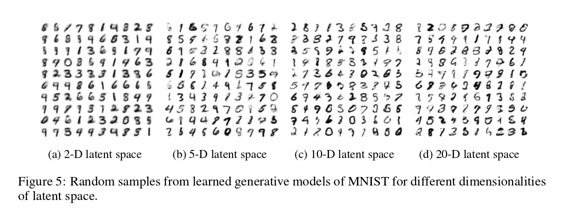
MNIST results

Frey Faces results

Dimension of latent variables

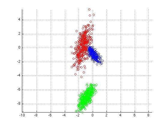
Mixture of Gaussians

Variational Inference

Variational inference is used in other areas… (TODO)

An example: Data from Mixture of Gaussians

• K mixture components, corresponding to normal distributions

• Means \(\boldsymbol{\mu}=\{\mu_1,...,\mu_K\} \sim \mathcal{N}(0, \sigma^2\boldsymbol{I})\)

• Mixture selection variable \(c_i \sim \text{Categorical}(1/K, ..., 1/K)\)

An example: Data from Mixture of Gaussians II

• Joint model \(\displaystyle p(\boldsymbol{\mu}, c_{1:n}, x_{1:n})=p(\boldsymbol{\mu}) \prod_{i=1}^n p(c_i)p(x_i|c_i,\boldsymbol{\mu})\)

• Each \(c_i\) has K options, and we have \(n\) data points, so \(O(K^n)\) to evaluate \(\displaystyle p(x_{1:n}) = \int p(\boldsymbol{\mu}, c_{1:n}, x_{1:n})\, d\boldsymbol{\mu}dc_{1:n}\)

An example: Data from Mixture of Gaussians III

• Each \(c_i\) has K options, and we have \(n\) data points, so \(O(K^n)\) to evaluate \(\displaystyle p(x_{1:n}) = \int p(\boldsymbol{\mu}, c_{1:n}, x_{1:n})\, d\boldsymbol{\mu}dc_{1:n}\)

• Takeaway message: can’t use direct estimation of the evidence \(p(x_{1:n})\)

• In this particular example we can use EM, but in general it assumes that you know \(p(\textbf{z}|\textbf{x})\)

Evidence Lower Bound (ELBO)

\[\begin{aligned} D_\text{KL}(q(\textbf{z})~||~p(\textbf{z}|\textbf{x})) &= \text{E}_{q}\left(\log\left(\frac{q(\textbf{z})}{p(\textbf{z} | \textbf{x})}\right)\right) \\ &= \text{E}_{q}(\log(q(\textbf{z}))) - \text{E}_{q}(\log(p(\textbf{z} | \textbf{x}))) \\ &= \text{E}_{q}(\log(q(\textbf{z}))) - \text{E}_{q}(\log(p(\textbf{z},\textbf{x}))) \\ &\hspace{12pt} + \text{E}_{q}(\log(p(\textbf{x}))) \\ &= \text{E}_{q}(\log(q(\textbf{z}))) - \text{E}_{q}(\log(p(\textbf{z},\textbf{x}))) \\ &\hspace{12pt} + \log(p(\textbf{x})) \\ &= -\text{ELBO}_{q}(\textbf{x}) + \log(p(\textbf{x})) \end{aligned}\]

Evidence Lower Bound (ELBO) II

Log-evidence:

\[\log(p(\textbf{x})) = D_\text{KL}(q(\textbf{z}) ~||~ p(\textbf{z} | \textbf{x})) + \text{ELBO}_q(\textbf{x})\]

Variational Inference \(\rightarrow\) find \(q(\textbf{z})\) that maximizes \(\text{ELBO}_q\)

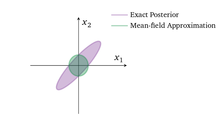
Mean-Field Approximation

• Simplification for posterior approximator \(q(\textbf{z})\):

• \(\displaystyle q(\textbf{z}) = \prod_j q_j(z_j)\)

• All latent variables \(z_j\) are mutually independent

• Each is governed by its own distribution \(q_j\)

• WHY? It makes the optimization easier (analytical gradients)

Mean-Field Approximation II

• WHY NOT? It fails to model correlations among latent variables, and underestimates variance

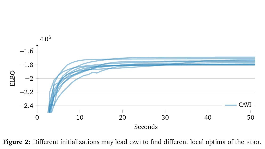
Optimization algorithms

• Algo \(\#1\): coordinate ascent along each latent variable of ELBO

• Main problem is that it evaluates ELBO on the entire dataset (not great for big data)

Optimization algorithms II

• Also susceptible to local minima

Optimization algorithms III

• Algo \(\#2\): stochastic optimization over all latent variables

• Uses the natural gradient to account for manifold on which distributions live

• Evaluates ELBO on single data points, or minibatches